Wingston Felix Ng’ambi1, Adamson Sinjani Muula2-4
- Health Economics and Policy Unit, Department of Health Systems and Policy, Kamuzu University of Health Sciences, Lilongwe, Malawi
2. Africa Centre of Excellence in Public Health and Herbal Medicine (ACEPHEM), Kamuzu University of Health Sciences, Blantyre, Malawi
3. Professor and Head, Department of Community and Environmental Health, School of Global and Public Health
4. President, ECSA College of Public Health Physicians, Arusha, Tanzania
Abstract
Introduction: Large-scale health surveys like the Demographic and Health Surveys (DHS) and WHO STEPS are essential for tracking health trends and guiding policies in low- and middle-income countries. However, when these datasets are imported into tools like R, they often lose crucial metadata, variable and value labels, turning clear categories into cryptic codes. This slows analysis, risks errors, and weakens data reuse.
Methods: We developed a reproducible workflow in R to import and process survey data while preserving variable and value labels. Using open-source packages such as haven, labelled, and tidyverse, we automated reading of datasets, extraction of metadata, replacement of codes with readable labels, and renaming of variables with full descriptions. The workflow was designed to be modular, easy to adapt, and accessible for analysts with basic R skills.
Results: We tested the workflow on the contraceptive use module from the 2015/16 Malawi DHS and the tobacco use module from Malawi’s Global Youth Tobacco Survey. Without our process, variables appeared as vague codes (e.g., v312) and responses as plain numbers. After applying our workflow, these were transformed into clear, labelled categories like “Injectable” or “Never Married.” Frequency tables generated from the cleaned data were easier to interpret and share. This automated approach saved several hours of manual recoding and reduced the risk of errors.
Conclusion: By maintaining metadata, our workflow improves transparency, reproducibility, and efficiency in digital health research. This supports better training, clearer communication, and more reliable use of health data for policy and program decisions.
Keywords: digital health, data harmonisation, metadata preservation, health surveys, reproducible research
Introduction
Routine health data collection in low- and middle-income countries (LMICs) provided information at regular intervals on services and activities delivered in health facilities1. Programs like the Demographic and Health Surveys (DHS) and WHO’s STEPwise approach to noncommunicable disease surveillance (STEPS) have become the backbone of health monitoring in these settings. These large-scale surveys gather rich information on population health, providing critical evidence for policy and program decisions2. As LMICs increasingly adopt digital health strategies, ensuring that this routine data retains essential metadata, such as variable and value labels, is key for transparent analyses, comparability across studies, and building reliable digital health systems. In digital health research, large-scale datasets such as the Demographic and Health Surveys (DHS)3 and WHO STEPwise surveys (STEPS)4 play a critical role in informing public health policy, monitoring health trends, and guiding decision-making. These datasets come with rich metadata, including variable labels that explain what each column represents, and value labels that describe coded responses5. However, when researchers import these files into statistical software like R, much of this metadata can be lost or mishandled. As a result, variables appear with cryptic names (e.g., v106, q102) and responses are shown as numbers without context (e.g., 1, 2, 3), making interpretation difficult and error-prone3.
Losing this metadata not only slows down analysis but also increases the risk of misinterpretation, especially for researchers who are new to the dataset or working in collaborative teams5. In digital health, where datasets are often reused across countries and over time, preserving labels ensures consistency, transparency, and reproducibility6. When labels are not retained, important details such as the meaning of categories, skip patterns, and question wording may be overlooked7. This can lead to incorrect analyses and conclusions, weakening the quality of research and its potential to inform policy or digital interventions8. This study addresses a common but under-discussed problem in digital health data management: the loss of variable and value labels during data import. By presenting a practical and reproducible workflow in R, we aim to support researchers, especially those in low- and middle-income countries, in maintaining data integrity from the start5. Our approach ensures that health data retains its meaning and context, making analysis more accurate, communication clearer, and results easier to share and validate. In doing so, this study contributes to better data stewardship and more reliable digital health evidence.
Methods
This study used the R programming language to develop a simple and reproducible workflow for importing and working with health survey data while preserving variable and value labels9,10. We relied on key packages including haven (to read SPSS and Stata files)11, labelled (to extract and handle metadata)12, and tidyverse (for data wrangling and cleaning)13. These tools were chosen because they are open-source, widely used in public health analytics, and compatible with a wide range of data formats14. Together, they allow researchers to retain the full descriptive structure of survey data, which is often lost in traditional data import steps.
To ensure the workflow is easy to replicate and adapt, all code was written in a modular format and documented using standard R scripts/markdown comments15. The process includes setting the file path, importing the dataset with all labels intact, extracting variable descriptions, flattening value labels into a readable format, and generating labelled frequency tables. Outputs such as CSVs for metadata and summary tables can be shared with collaborators or used directly in reports. The script is adaptable to any dataset and is designed to be used by analysts with basic R skills.
As proof of concept, we applied the workflow to two common modules: the contraceptive use section of the 2015/6 Malawi DHS (MWIR7HFL.DTA) from Measure DHS and the tobacco consumption section of a Global Youth Tobacco Survey (MWI2009.dta) from NCD monitor. In both cases, we successfully preserved metadata that clearly defined coded responses such as types of contraceptive methods and levels of alcohol use. By maintaining the link between values and their labels, we improved the interpretability of results and reduced the risk of analytic errors10. These examples highlight how the approach can be used to support accurate, reproducible, and policy-relevant analysis in digital health studies15.
Ethical consideration
This study did not involve the collection of new data from human participants. Instead, we used publicly available datasets from the 2015/16 Malawi Demographic and Health Survey (DHS (https://dhsprogram.com/data/dataset_admin/login_main.cfm) and the Malawi Global Youth Tobacco Survey (https://extranet.who.int/ncdsmicrodata/index.php/catalog/147/variable/V212). These datasets were fully anonymized, with all personal identifiers removed before we accessed them. We followed all data use agreements set by the data custodians. Our work mainly served as a technical proof of concept to show how metadata can be preserved and linked to coded values, making analyses clearer and reducing mistakes. By doing this, we aimed to support more transparent and trustworthy research that can inform health policies without compromising participant privacy.
Results
Workflow to preserve variable and value labels in Stata, SPSS, and SAS datasets
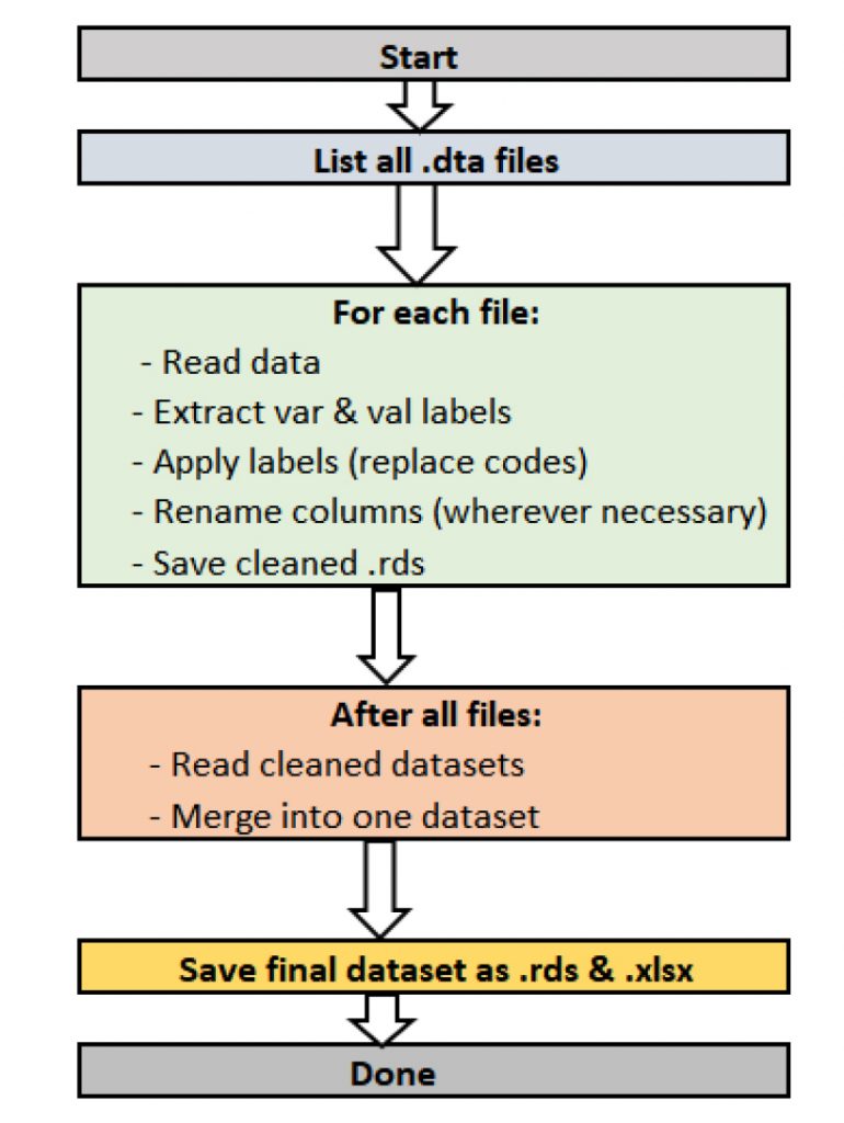
To preserve variable and value labels when working with datasets from Stata, SPSS, or SAS, start by using specialized R packages that can handle these formats without stripping metadata used the workflow in Figure 1. The haven package is especially useful because it reads .dta (Stata), .sav (SPSS), and .sas7bdat (SAS)11 files while keeping variable labels (describing what each column means) and value labels (explaining coded responses). Once imported, you can use the labelled package to easily view, manage, and convert these labels 12. For instance, you can extract variable descriptions into a separate table for documentation or apply value labels directly, so coded numbers instantly show up as clear categories like “Married” or “Never smoked.” After reading in and cleaning each dataset, the workflow continues by applying labels to the data so they become part of summaries, plots, and exported files. Before exporting, rename columns to include full variable labels for better readability outside R. Finally, save the fully labelled dataset as an RDS file to preserve the structure for future analysis, or write it out to Excel or CSV along with a key that lists all variable and value meanings. This approach ensures your data always carries the full context, making it easier to interpret, share, and trust; whether it originally came from Stata, SPSS, or SAS.
Merits of proposed workflow
The workflow revealed significant differences in how data appears and is understood before and after label preservation. For instance, in the contraceptive use module of the DHS dataset, the variable v312 appears as a numeric field without labels when imported using default methods. Without labels, values such as 1, 2, or 3 are meaningless to analysts unfamiliar with the coding. After applying the proposed workflow, those same values are automatically linked to their full descriptions, such as “Pill,” “IUD,” or “Injectable,” allowing for accurate interpretation without manual code lookups or referencing external codebooks (see Figure 2 (code: MMJ_Paper_Script_Labelling_Values_13_July_2025_FINAL.R), Figure 3 (code: MMJ_Paper_Script_Labelling_Values_13_July_2025_FINAL.R) and Figure 4 (code: MMJ_Paper_Script_13_July_2025_FINAL.R)).
Figure 2: A sample of the extracted value labels from the Malawi 2015/6 women dataset
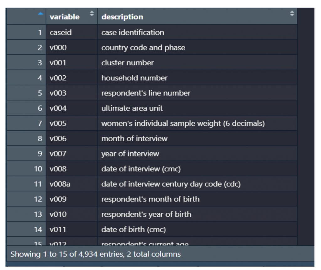
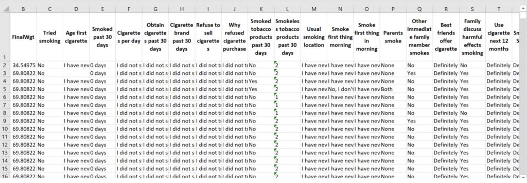
Figure 3: Combination of data with both variable and value labels for the 2009 Malawi Global Youth Tobacco Survey
We also compared frequency tables generated with and without labels. Without labels, output tables contain only numbers, which require the user to cross-check codes in the original questionnaire or recode them manually. In contrast, when using the labelled data workflow, frequency tables present clean, readable summaries such as “Never Married,” “Married,” or “Widowed,” making it immediately clear what the distributions represent. This clarity improves the usability of outputs for presentations, reports, and peer-reviewed publications, especially for audiences with limited statistical training.
Option A: Frequency tables with vs. without labels
Without labels
Code:
vars_to_freq <- c(“v502”, “v025”, “v106”)
# Create output folder if needed
if (!dir.exists(“Output”)) dir.create(“Output”)
for (var in vars_to_freq) {
if (var %in% names(women)) {
# Use table() to count values
tbl <- table(women[[var]])
# Turn into data frame
freq_table <- as.data.frame(tbl)
names(freq_table) <- c(“value”, “count”)
# Calculate percentage
freq_table$percent <- round(100 * freq_table$count / sum(freq_table$count), 1)
# Save CSV
write_csv(freq_table, paste0(“Output/frequency_”, var, “.csv”))
print(paste(“Saved frequency table for”, var))
} else {
warning(paste(“Variable”, var, “not found in dataset”))
}
}
Output:
V502: Marital status
With labels
Code:
vars_to_freq <- c(“v502”, “v025”, “v106”) # You may need to adjust names based on actual dataset
# Function to create and save frequency table for each variable
for (var in vars_to_freq) {
if (var %in% names(women)) {
freq_table <- women %>%
mutate(temp = as_factor(.data[[var]])) %>%
count(temp, name = “count”) %>%
mutate(percent = round(100 * count / sum(count), 1)) %>%
rename(label = temp)
write_csv(freq_table, paste0(“frequency_”, var, “.csv”))
} else {
warning(paste(“Variable”, var, “not found in dataset”))
}
}
Ouput
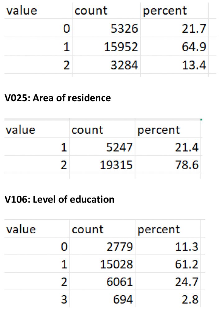
V502: Marital status
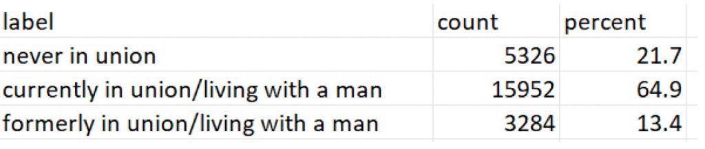
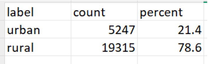
V025: Area of residence
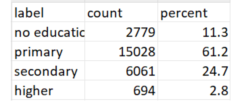
V106: Level of education
Option B: Frequency tables for the variable and value labels transformed
The workflow not only improves readability but also reduces time and errors. Manual recoding and referencing of external codebooks are time-consuming, particularly in large datasets with hundreds of variables. By automating label extraction and applying consistent formatting, our approach helps analysts avoid common mistakes such as mislabeling variables or misclassifying categories. In our case examples, label preservation and formatting saved several hours of manual work and eliminated the need for guesswork or repeated code verification, making the data analysis process more efficient and reliable.
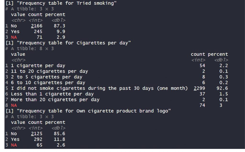
After running the code (MMJ_Paper_Script_13_July_2025_FINAL.R) on mwi2009.dta, we generated a dataset with both variable and value labels called merged_data.csv. Then we run the code below.
# Make sure packages are loaded
library(dplyr)
library(readr)
# List of variables
vars_to_summarise <- c(“Tried smoking”, “Cigarettes per day”, “Own cigarette product brand logo”)
# Loop over each variable
for (var in vars_to_summarise) {
freq_table <- merged_data %>%
count(!!sym(var), name = “count”) %>%
mutate(percent = round(100 * count / sum(count), 1)) %>%
rename(value = !!sym(var))
# Print to console
print(paste(“Frequency table for”, var))
print(freq_table)
}
This code produced the following output:
Demerits of the proposed workflow
While this workflow greatly improves efficiency and helps keep data clear and well-labelled, it does come with a few downsides. It relies heavily on R and specific packages, which means users need at least basic R skills to run or adapt it. If variable names or label structures change too much across files, the automated steps might not work perfectly and still require manual checks. Also, since it saves outputs in R-specific formats like .rds, people using other software may need extra steps to read the data. In short, while the workflow reduces many errors and saves time, it still needs some technical know-how and careful oversight to handle unusual or inconsistent datasets.
Converting the data to show variable and value labels
Converting the data to show both variable and value labels was a crucial part of our process. Using our R script, we carefully unpacked each dataset to pull out the hidden meanings behind cryptic codes and column names 5 12. We replaced raw numeric codes with their real-world labels, like turning a plain 1 or 0 into clear categories such as “Yes” or “No.” At the same time, we renamed the columns to display full variable labels, so instead of vague names like q101, we now had straightforward titles like “Current tobacco use.” This not only made the data far easier to read and understand but also reduced the chance of mistakes during analysis. By doing this, we transformed a dense, coded dataset into a clean, human-friendly table that clearly tells the story behind the numbers.
Extension when combining data from multiple surveys
To prepare multiple survey datasets for easy analysis, we first set up a workflow in R to automatically read and clean all .dta files in a specified folder. Using packages like haven, dplyr, tidyr, and labelled, the script reads each dataset, extracts the variable labels (like “Type of tobacco used”) and the value labels (like 1 = “Yes”, 0 = “No”), and saves these as separate files13. It then attaches the value labels back to the actual data, replacing raw codes with meaningful descriptions. This makes the dataset more readable and minimizes the chance of misinterpreting codes16. To avoid losing context, the script also renames the columns using their full variable labels, keeping them informative even outside specialized software like Stata17. Once all individual datasets are cleaned and labelled, the script gathers them into one combined file16. Before merging, it converts key survey design identifiers like stratum and psu into character type to prevent merge errors. The final merged dataset is then saved both as an RDS file for future analysis in R and as an Excel file for easy sharing17. This automated process ensures consistency, saves time, and gives a tidy dataset ready for analysis or reporting18,19.
Below are the key code snippets:
- Loop through all
.dtafiles and process them
dta_files <- list.files(data_dir, pattern = “\\.dta$”, full.names = TRUE)
walk(dta_files, process_file)
- Inside
process_file, replace codes with labels and rename columns
# Apply value labels
for (var in names(data)) {
val_lab <- value_labels_long %>% filter(variable == var)
if (nrow(val_lab) > 0) {
lookup <- setNames(as.character(val_lab$label), val_lab$code)
data[[var]] <- recode(as.character(data[[var]]), !!!lookup)
}
}
# Rename columns with variable labels
data <- data %>% rename_with(~ rename_vector[.x], .cols = names(data))
- Merge all cleaned datasets and export
cleaned_files <- list.files(data_dir, pattern = “_cleaned\\.rds$”, full.names = TRUE)
merged_data <- map_dfr(cleaned_files, function(file) {
df <- readRDS(file)
df <- df %>% mutate(across(any_of(c(“stratum”, “psu”)), as.character))
}, .id = “source_file”)
saveRDS(merged_data, file = file.path(data_dir, “gtys_2000_2021.rds”))
write_xlsx(merged_data, path = file.path(data_dir, “gtys_2000_2021.xlsx”))
Harmonisation of datasets
When working with surveys collected across different years or from multiple sources, the data often comes in slightly different shapes9. Variable names might change, codes for answers may be inconsistent, or important labels could be missing. Without careful cleaning, merging these datasets can easily produce errors or misleading results. That’s why data harmonisation is a key step before any analysis. In this work, we automated harmonisation using R10. Each dataset was first read in and cleaned by replacing raw codes (like 1, 2, 3) with their actual meanings (like “Male”, “Female”, “Other”), based on the value labels stored in the original files. We also ensured that the columns carried clear descriptive names by applying the variable labels. After each individual dataset was cleaned and saved, we combined them into one big file. Before merging, we converted critical survey design identifiers such as stratum and psu into character type to keep things consistent. This entire process helped us standardise multiple datasets, making sure they spoke the same “language”. The result was a single tidy dataset that was ready for robust, error-free analysis and easy interpretation16.
Time saved or errors avoided
One of the biggest wins from this approach was the time it saved and the errors it helped us avoid. By automating the process of applying variable and value labels5, we skipped the tedious and error-prone manual recoding that often leads to mistakes19. This meant we did not have to keep checking codebooks or guessing what each number stood for. With clearly labelled data from the start, we avoided misclassifying responses or running faulty analyses based on misunderstood codes9. In short, this streamlined workflow not only cut down hours of repetitive work but also gave us cleaner results we could trust.
Discussion
Preserving variable and value labels in health datasets is more than a technical concern it directly affects the reproducibility and integrity of digital health research20,21. Inconsistent or missing metadata leads to misinterpretation, delays in analysis, and difficulties in replicating findings22. This is particularly problematic in digital health, where data-driven decisions influence policies, resource allocation, and program design23. Our approach supports reproducible research by ensuring that survey data maintains its full descriptive structure throughout the analytic workflow, allowing others to understand, verify, and replicate results with confidence.
The implications for training are also significant24. Many researchers and students in low- and middle-income countries work with large datasets like DHS or STEPS25,26 but often lack access to proprietary software or detailed technical support. Providing a reproducible R workflow that maintains metadata helps bridge this gap10. It makes these datasets more accessible and easier to use in teaching settings, enabling new users to focus on data interpretation rather than data cleaning or codebook decoding. This contributes to building local capacity in data science and strengthens the pipeline of skilled analysts in digital health27.
Moreover, preserving labels enhances data sharing and collaboration12. When datasets are stripped of labels, shared files become harder to understand or reuse, especially across teams or institutions 25,28. By exporting variable descriptions and value labels alongside the cleaned dataset, researchers can ensure that collaborators and secondary users interpret the data correctly29. This is especially valuable in multi-country or multi-year studies, program evaluations, or open data platforms, where keeping consistency and meaning across datasets is essential.
Finally, this approach supports the broader goals of open science 30, 31, 32. By using open-source tools and emphasizing transparency in the data preparation process, we help make digital health research more inclusive and efficient 33 34. Analysts can document their data workflows clearly, share code and metadata publicly, and contribute to more equitable and trustworthy use of health data 35,36. As the demand for real-time data and reproducible evidence grows, workflows like this one become increasingly important for the future of global digital health.
We recommend that researchers and analysts working with health survey data adopt this workflow early in their projects to maintain data clarity and avoid time-consuming manual relabelling later. It is best to keep a consistent folder structure, document each step, and always save intermediate outputs with clear filenames 37. This makes it easier to track changes and revisit your work if needed. We also suggest sharing both the cleaned datasets and accompanying metadata files, so collaborators can understand exactly what each variable and value means without digging into codebooks.
All the tools used in this workflow; haven11, labelled12, dplyr 38, and tidyr13; are freely available as R packages on CRAN. The full scripts that power this process, including functions to read, label, clean, and merge datasets, are provided in well-commented R file that can be easily adapted to different surveys. To make this workflow even more accessible, we also highlight the opportunity to develop equivalent scripts in Python using libraries such as pandas, pyreadstat, and numpy39. This would allow analysts more familiar with Python to perform the same steps of importing data, preserving variable and value labels, recoding, and merging multiple survey datasets40. The R script has been included in the paper as supplementary material. This way, other teams can replicate the workflow, adapt it to their own data, develop Python versions, and contribute further improvements.
Author contributions
WFN= Conceptualisation and drafting the paper and code. ASM=Reviewing the paper and the code. Both authors reviewed and approved the paper together with the code.
Competing interest
None
Funding
None
References
1. Hung, Y. W., Hoxha, K., Irwin, B. R., Law, M. R. & Grépin, K. A. Using routine health information data for research in low- and middle-income countries: a systematic review. BMC Health Serv. Res. 20, 790 (2020).
2. Institute of Medicine (US) Committee on Assuring the Health of the Public in the 21st Century. The Future of the Public’s Health in the 21st Century. Washington (DC): National Academies Press (US); 2002. 2, Understanding Population Health and Its Determinants. Available from: Https://Www.Ncbi.Nlm.Nih.Gov/Books/NBK221225/.
3. Croft, Trevor N., Allen, Courtney K., Zachary, Blake W., et al. 2023. Guide to DHS Statistics. Rockville, Maryland, USA: ICF.
4. Riley, L. et al. The World Health Organization STEPwise Approach to Noncommunicable Disease Risk-Factor Surveillance: Methods, Challenges, and Opportunities. Am. J. Public Health 106, 74–78 (2016).
5. Buttliere, B. Adopting standard variable labels solves many of the problems with sharing and reusing data. Methodol. Innov. 14, 205979912110266 (2021).
6. Condon, P., Simpson, J. & Emanuel, M. Research data integrity: A cornerstone of rigorous and reproducible research. IASSIST Q. 46, (2022).
7. Arslan, R. C. How to Automatically Document Data With the codebook Package to Facilitate Data Reuse. Adv. Methods Pract. Psychol. Sci. 2, 169–187 (2019).
8. Shreffler J, Huecker MR. Common Pitfalls In The Research Process. [Updated 2023 Mar 6]. In: StatPearls [Internet]. Treasure Island (FL): StatPearls Publishing; 2025 Jan-. Available from: Https://Www.Ncbi.Nlm.Nih.Gov/Books/NBK568780/.
9. Kołczyńska, M. Combining multiple survey sources: A reproducible workflow and toolbox for survey data harmonization. Methodol. Innov. 15, 62–72 (2022).
10. Shimizu, I. & Ferreira, J. C. Losing your fear of using R for statistical analysis. J. Bras. Pneumol. Publicacao Of. Soc. Bras. Pneumol. E Tisilogia 49, e20230212 (2023).
11. Wickham H, Miller E, Smith D (2025). haven: Import and Export ‘SPSS’, ‘Stata’ and ‘SAS’ Files. R package version 2.5.5, https://haven.tidyverse.org. in.
12. Larmarange J (2025). _labelled: Manipulating Labelled Data_. doi:10.32614/CRAN.package.labelled <https://doi.org/10.32614/CRAN.package.labelled>, R package version 2.14.1, <https://CRAN.R-project.org/package=labelled>. in.
13. Wickham, H. et al. Welcome to the Tidyverse. J. Open Source Softw. 4, 1686 (2019).
14. Daswito, R., Besral, B. & Ilmaskal, R. Analysis Using R Software: A Big Opportunity for Epidemiology and Public Health Data Analysis. J. Health Sci. Epidemiol. 1, 1–5 (2023).
15. Peikert, A., van Lissa, C. J. & Brandmaier, A. M. Reproducible Research in R: A Tutorial on How to Do the Same Thing More Than Once. Psych 3, 836–867 (2021).
16. Wickham, H. Tidy data. Am. Stat. 14, (2014).
17. Buttliere, B. Adopting standard variable labels solves many of the problems with sharing and reusing data. Methodol. Innov. 14, 20597991211026616 (2021).
18. Hosseinzadeh, M. et al. Data cleansing mechanisms and approaches for big data analytics: a systematic study. J. Ambient Intell. Humaniz. Comput. 14, 1–13 (2021).
19. Nguyen, T., Nguyen, H.-T. & Nguyen-Hoang, T.-A. Data quality management in big data: Strategies, tools, and educational implications. J. Parallel Distrib. Comput. 200, 105067 (2025).
20. Condon, P., Simpson, J. & Emanuel, M. Research data integrity: A cornerstone of rigorous and reproducible research. IASSIST Q. 46, (2022).
21. Syed, R. et al. Digital Health Data Quality Issues: Systematic Review. J. Med. Internet Res. 25, e42615 (2023).
22. Cai, L. & Zhu, Y. The Challenges of Data Quality and Data Quality Assessment in the Big Data Era. Data Sci. J. 14, (2015).
23. Ulrich, H. et al. Understanding the Nature of Metadata – A Systematic Review. J. Med. Internet Res. (2020) doi:10.2196/25440.
24. Custer, G. F., van Diepen, L. T. A. & Seeley, J. Student perceptions towards introductory lessons in R. Nat. Sci. Educ. 50, e20073 (2021).
25. Witter, S., Sheikh, K. & Schleiff, M. Learning health systems in low-income and middle-income countries: exploring evidence and expert insights. BMJ Glob. Health 7, (2022).
26. Riley, L. et al. The World Health Organization STEPwise Approach to Noncommunicable Disease Risk-Factor Surveillance: Methods, Challenges, and Opportunities. Am. J. Public Health 106, 74–78 (2016).
27. Botero-Mesa, S. et al. Leveraging human resources for outbreak analysis: lessons from an international collaboration to support the sub-Saharan African COVID-19 response. BMC Public Health 22, (2022).
28. Buttliere, B. Adopting standard variable labels solves many of the problems with sharing and reusing data. Methodol. Innov. 14, 205979912110266 (2021).
29. Arslan, R. C. How to Automatically Document Data With the codebook Package to Facilitate Data Reuse. Adv. Methods Pract. Psychol. Sci. 2, 169–187 (2019).
30. Williams, T. & Taqa, A. Open Science Initiatives: Advancing Collaborative and Transparent Scientific Research. 8, 3006–2853 (2020).
31. Chiware, E. R. T. & Lockhart, J. Open Science. in Encyclopedia of Libraries, Librarianship, and Information Science (First Edition) (eds. Baker, D. & Ellis, L.) 440–446 (Academic Press, Oxford, 2025). doi:10.1016/B978-0-323-95689-5.00061-4.
32. Van Vaerenbergh, Y., Hazée, S. & Zwienenberg, T. J. Open Science: A Review of Its Effectiveness and Implications for Service Research. J. Serv. Res. 10946705251338461 (2025) doi:10.1177/10946705251338461.
33. Fitzpatrick, P. J. Improving health literacy using the power of digital communications to achieve better health outcomes for patients and practitioners. Front. Digit. Health 5, 1264780 (2023).
34. Chidera, V. et al. Data analytics in healthcare: A review of patient-centric approaches and healthcare delivery. World J. Adv. Res. Rev. 21, 1750–1760 (2024).
35. Cascini, F. et al. Health data sharing attitudes towards primary and secondary use of data: a systematic review. EClinicalMedicine 71, 102551 (2024).
36. Ugochukwu, A. I. & Phillips, P. W. B. Open data ownership and sharing: Challenges and opportunities for application of FAIR principles and a checklist for data managers. J. Agric. Food Res. 16, 101157 (2024).
37. Smith A. (2018). An Example Directory Structure. GitHub. Retrieved from Https://Github.Com/Aosmith16/Aosmith/Blob/Master/Content/Post/2018-10-29-an-Example-Directory-Structure.Rmd.
38. Wickham H, François R, Henry L, Müller K, Vaughan D (2025). Dplyr: A Grammar of Data Manipulation. R Package Version 1.1.4, Https://Dplyr.Tidyverse.Org.
39. Kabir, M. A., Ahmed, F., Islam, M. M. & Ahmed, Md. R. Python For Data Analytics: A Systematic Literature Review Of Tools, Techniques, And Applications. Acad. J. Sci. Technol. Eng. Math. Educ. 4, 134–154 (2024).
40. Kebede Gebre, K. & Wesenu, M. Statistical Data Analysis Using Python. (2024).