A Practical Guide to Key Considerations in Logistic Regression for Clinical and Public Health Research: R tutorial

Wingston Felix Ng’ambi¹, Cosmas Zyambo, Adamson Sinjani Muula^3-5

Health Economics and Policy Unit, Department of Health Systems and Policy, Kamuzu University of Health Sciences, Lilongwe, Malawi
Africa Centre of Excellence in Public Health and Herbal Medicine (ACEPHEM), Kamuzu University of Health Sciences, Blantyre, Malawi
Department of Public Health and Family Medicine, University of Zambia, Lusaka, Zambia
Professor and Head, Department of Community and Environmental Health, School of Global and Public Health
President, ECSA College of Public Health Physicians, Arusha, Tanzania

Abstract

Logistic regression is one of the most widely used statistical methods in clinical and public health research, especially for analysing binary outcomes such as disease presence, treatment uptake, or health behaviour change. While its use appears straightforward, important methodological decisions made during data preparation, model specification, and interpretation can substantially influence findings and their policy relevance. This paper offers a practical, step-by-step guide to key considerations in logistic regression, tailored for clinical and public health researchers. Drawing from applied examples in infectious diseases, non-communicable diseases, and health services research, we highlight common pitfalls and best practices for variable selection, model diagnostics, handling missing data, assessing fit, and presenting results. The guide aims to bridge the gap between statistical theory and real-world application, equipping researchers to produce more robust, transparent, and policy-relevant evidence.

Key Words

Logistic regression, Clinical research, Public Health, infectious diseases, non-communicable diseases, health services research

Introduction

Logistic regression is one of the most widely used statistical tools in clinical and public health research¹. Its versatility, interpretability, and capacity to model binary outcomes make it an indispensable method in epidemiology, health services research, and health policy analysis³. In clinical and public health, binary outcomes are common⁸; for example, whether an individual is vaccinated, whether a patient adheres to treatment, or whether a pregnant woman delivers in a health facility. Logistic regression allows researchers to examine the relationship between such outcomes and multiple predictors, while adjusting for potential confounding factors⁹. In global health research contexts, logistic regression underpins analyses from flagship datasets such as the Demographic and Health Surveys (DHS), the Multiple Indicator Cluster Surveys (MICS), the World Health Organization’s STEPS surveys, and disease-specific surveys such as the Population-based HIV Impact Assessments (PHIA). These data sources are often the backbone of national health policy reviews, donor-funded programme evaluations, and academic studies ¹⁰. For instance, logistic regression has been used to identify determinants of HIV testing uptake across sub-Saharan Africa, factors influencing childhood immunisation in South Asia, and socio-economic predictors of maternal health service use in Latin America. Despite its broad adoption, the method is often misapplied or under-reported. Studies may omit critical details about variable selection, ignore checks for key assumptions such as linearity in the logit, or misinterpret odds ratios as risk ratios. Where many datasets are collected using complex survey designs, a frequent oversight is failing to account for clustering, stratification, and sampling weights¹¹. This can lead to biased estimates, misleading standard errors, and ultimately, practice and policy recommendations that are not supported by the data¹².

The gap between statistical theory and its practical application is a constant threat in understanding research findings. Researchers may be constrained by small sample sizes¹³, incomplete data¹⁴, or limited access to statistical training and software¹⁵. These challenges can result in oversimplified analyses that miss important interactions or produce unstable estimates¹⁶. For example, a study examining determinants of hypertension treatment in a country may exclude socio-economic variables because of missing data, or might not test for interaction effects between age and sex, thereby overlooking potentially important policy insights. The aim of this paper is to provide a practical, step-by-step guide to key considerations when applying the logistic regression in public health research, with a specific focus on contexts relevant to both global and African health studies. This guide bridges the gap between statistical best practice and the realities of working with large-scale survey data, health facility datasets, and programmatic monitoring systems. It is written for applied researchers, programme evaluators, postgraduate students, and public health practitioners who may not be statisticians by training but who regularly use logistic regression to generate evidence for decision-making.

Data sets analysed

Throughout the paper, we combine statistical principles with worked examples in R, using real-world datasets from both global and African sources. Examples include:

– Predictors of full immunisation among children aged 12–23 months using the Malawi Demographic and Health Survey (DHS) 2015–16 data MDHS 2015-2016. Below is the code that creates the dhs_mw dataset for analysis.

# Always set working directory to the current project folder
setwd(getwd())

# Load required packages ———————————————

library(haven) # for reading Stata (.dta) files like DHS datasets
library(dplyr) # for data wrangling (filtering, mutating, selecting)

Attaching package: ‘dplyr’

The following objects are masked from ‘package:stats’:

filter, lag

The following objects are masked from ‘package:base’:

intersect, setdiff, setequal, union

library(labelled) # for handling variable/value labels from DHS
library(mice) # for multiple imputation of missing values

Attaching package: ‘mice’

The following object is masked from ‘package:stats’:

filter

The following objects are masked from ‘package:base’:

cbind, rbind

library(survey) # for survey-weighted analyses (logistic regression)

Loading required package: grid

Loading required package: Matrix

Loading required package: survival

Attaching package: ‘survey’

The following object is masked from ‘package:graphics’:

dotchart

# 1. Load DHS dataset ————————————————

dhs_mw <- read_dta(“MWKR7AFL.DTA”)
# Reads the DHS Malawi Kids Recode file (KR) in Stata format (.dta).
# The object ‘dhs_mw’ now contains the full DHS dataset for analysis.

# 2. Select children age 12–23 months ——————————–

dhs_mw <- dhs_mw %>%
filter(b8 >= 1 & b8 <= 2)
# b8 = age of child in years
# We restrict the sample to children 12–23 months old, since they are
# expected to have completed all basic vaccinations.

# 3. Define full immunisation outcome ——————————–

dhs_mw <- dhs_mw %>%
mutate(
    full_immunisation = case_when(
      # child fully immunised if all required vaccines are 1,2,3
      h2 %in% c(1,2,3) &   # BCG
      h3 %in% c(1,2,3) &   # DPT1
      h4 %in% c(1,2,3) &   # DPT2
      h5 %in% c(1,2,3) &   # DPT3
      h6 %in% c(1,2,3) &   # Polio1
      h7 %in% c(1,2,3) &   # Polio2
      h8 %in% c(1,2,3) &   # Polio3
      h9 %in% c(1,2,3) &   # Measles
      h9a %in% c(1,2,3)    # Sometimes measles2 / rubella etc depending on DHS round
      ~ 1,
      TRUE ~ 0
    )
)
# Creates a binary outcome variable ‘full_immunisation’.
# A child is coded 1 if they received all required vaccines:
#   BCG, 3 doses of DPT, 3 doses of polio, and measles.
# Otherwise, coded as 0.
# NOTE: variable names (bcg, dpt1, etc.) may differ in your DHS file
# and need to be checked.

# 4. Recode predictors and keep analysis variables ——————-

dhs_mw <- dhs_mw %>%
mutate(
    child_age = b8,   # keep child age in months as continuous predictor

    mother_education = factor(v106,                       # mother’s education level
                              levels = c(0,1,2,3),
                              labels = c(“none”,”primary”,”secondary”,”higher”)),

    wealth_quintile = factor(v190,                        # household wealth quintile
                             levels = 1:5,
                             labels = c(“poorest”,”poorer”,”middle”,”richer”,”richest”)),

   urban = ifelse(v025 == 1, 1, 0),                      # place of residence
    # v025 = type of residence (1=urban, 2=rural).
    # We recode to binary (1=urban, 0=rural).

    mother_age = factor(v013,                             # mother’s age group
                        levels = 1:7,
                        labels = c(“15-19″,”20-24″,”25-29”,
                                   “30-34″,”35-39″,”40-44″,”45-49”)),

    region = factor(v024,                                 # region of residence
                  levels = c(1,2,3),
                    labels = c(“Northern”,”Central”,”Southern”)),

    cluster = v021,    # cluster (primary sampling unit, PSU)
    strata = v022,    # survey strata
    weight = v005 / 1000000   # sample weight (normalize by 1,000,000 as per DHS)
) %>%
select(full_immunisation, child_age, mother_education, mother_age,
         wealth_quintile, urban, region, cluster, strata, weight)
# After recoding, we keep only the variables relevant for the analysis.

#Dealing with data types so that we are able to run all the commands perfectly
dhs_mw$mother_education <- factor(dhs_mw$mother_education,
                                  levels = c(“none”, “primary”, “secondary”, “higher”))
dhs_mw$child_age <- factor(dhs_mw$child_age, levels = c(1,2))
dhs_mw$urban <- factor(dhs_mw$urban, levels = c(0,1))
dhs_mw$wealth_quintile <- factor(dhs_mw$wealth_quintile,
                                 levels = c(“poorest”, “poorer”, “middle”, “richer”, “richest”))

By grounding the discussion in real datasets, we demonstrate how key considerations such as outcome coding, variable selection, model diagnostics, and interpretation translate into practical steps. We also highlight common pitfalls and provide recommendations to ensure logistic regression results are robust, transparent, and practice and policy-relevant. In doing so, this paper aims to demystify logistic regression for applied public health research, contexts where data complexity and policy urgency demand both statistical rigour and pragmatic decision-making.

Step-by-step guide to key considerations

This section gives a hands-on, practical walk through the most important choices you will make when using logistic regression in clinical and public health work. Each part explains why the step matters, shows common mistakes, and gives short R code you can copy and adapt. We use short, clear language, one idea per sentence, and real public health examples from Africa and elsewhere.

Step 1: Define the research question A clear question is the most important start. Ask, what is the exact outcome. Ask, is it naturally binary, or am I forcing a binary split. Be explicit about whether your aim is explanation, causal inference, or prediction¹⁷. Each aim needs a slightly different approach. A precise research question is the foundation of any analysis. This requires clear specification of the outcome, with attention to whether it is naturally binary or whether dichotomisation is being imposed on a continuous or ordinal variable, which can reduce information¹⁸. Equally important is explicit definition of the analytic aim. Explanatory analyses prioritise identifying associations and patterns between variables, whereas causal inference focuses on estimating the effect of an exposure or intervention under defined assumptions¹⁹. In contrast, prediction models aim to maximise accuracy in forecasting outcomes, often using machine learning methods that prioritise performance over interpretability. Distinguishing between these aims at the outset ensures alignment between research design, choice of methods, and interpretation of results²⁰.

Example, explanatory question: “What factors predict facility delivery in rural Malawi?” Here you want effect estimates that adjust for confounding. Use odds ratios carefully, and consider risk differences for policy clarity.

Example, predictive question: “Can we predict which children will be fully immunised in Malawi?” Here you focus on discrimination and calibration, you care less about causal interpretation.

Practical checks, before modelling: Before starting any modelling, it is important to carry out some practical checks to ensure your analysis is robust. First, inspect the frequency of your outcome: very rare events or extremely common outcomes can pose challenges for standard regression methods and may require alternative approaches or careful interpretation. Second, decide on your reference category for categorical variables, code it clearly (for example, 0 versus 1), and document this choice explicitly in your methods section. Doing so improves transparency, reproducibility, and clarity for readers, reviewers, and policymakers who may rely on your findings.

R, quick checks:

# check outcome distribution
table(dhs_mw$full_immunisation)

0 1
5626 874

prop.table(table(dhs_mw$full_immunisation))

0 1
0.8655385 0.1344615

Step 2: Data preparation Outcome coding: This section addresses outcome coding, predictor coding, handling of missing data, survey design features, and simple data transformations. For outcome coding, clarity is essential. Outcomes should be coded consistently, often using 0 and 1 to indicate absence and presence of the event, respectively³. It is critical to state explicitly which value represents the event of interest. For example, in the Malawi Demographic and Health Survey (DHS) child immunisation dataset, the outcome can be coded as 1 = fully immunised and 0 = not fully immunised. Such explicit coding not only reduces ambiguity but also facilitates reproducibility and comparability across analyses. R, example:

table(dhs_mw$full_immunisation, useNA = “ifany”)

0 1
5626 874

Predictor coding: For predictor coding, simplicity and interpretability should guide decisions. Categories should be meaningful and analytically relevant, while avoiding excessive fragmentation into many small groups with very few observations, which can compromise statistical power and model stability²¹. When continuous variables are used in interaction terms, centring them around their mean is recommended, as this improves the interpretability of regression coefficients and reduces multicollinearity²².

Missing data: For missing data, exploration of patterns is the first step. It is important to assess whether data are missing completely at random (MCAR), missing at random (MAR), or missing not at random (MNAR), as each mechanism has different implications for analysis¹⁴. In many health survey settings, multiple imputation provides a robust approach for handling missingness and yields less biased estimates compared to ad hoc methods²⁵. Complete-case analysis should be avoided when the proportion of missing data is greater than 10%, as this can reduce statistical power and lead to biased results if the missingness is not completely at random²⁶.

R, example with mice:

library(mice)
# md.pattern(dhs_mw) # Our data is completely observed with no missing data
imp <- mice(dhs_mw %>% select(full_immunisation, child_age, mother_education, wealth_quintile, urban),
m = 5, method = ‘pmm’, seed = 123)

iter imp variable
1   1
1   2
1   3
1   4
1   5
2   1
2   2
2   3
2   4
2   5
3   1
3   2
3   3
3   4
3   5
4   1
4   2
4   3
4   4
4   5
5   1
5   2
5   3
5   4
5   5

mod_imp <- with(imp, glm(full_immunisation ~ child_age + mother_education + wealth_quintile + urban,
family = binomial))
pool(mod_imp)

Class: mipo    m = 5
                        term m    estimate        ubar b           t dfcom
1                (Intercept) 5 -2.02286323 0.017112417 0 0.017112417 6490
2                 child_age2 5 -0.17364443 0.005336868 0 0.005336868 6490
3    mother_educationprimary 5 0.04161282 0.014670901 0 0.014670901 6490
4 mother_educationsecondary 5 0.11769675 0.021149348 0 0.021149348 6490
5     mother_educationhigher 5 -0.03311987 0.094604028 0 0.094604028 6490
6      wealth_quintilepoorer 5 0.13756188 0.013136974 0 0.013136974 6490
7      wealth_quintilemiddle 5 0.17057447 0.013670904 0 0.013670904 6490
8      wealth_quintilericher 5 0.31267124 0.014138052 0 0.014138052 6490
9     wealth_quintilerichest 5 0.29185892 0.019885581 0 0.019885581 6490
10                    urban1 5 0.10163447 0.012979206 0 0.012979206 6490
         df riv lambda          fmi
1 6487.247   0      0 0.0003081547
2 6487.247   0      0 0.0003081547
3 6487.247   0      0 0.0003081547
4 6487.247   0      0 0.0003081547
5 6487.247   0      0 0.0003081547
6 6487.247   0      0 0.0003081547
7 6487.247   0      0 0.0003081547
8 6487.247   0      0 0.0003081547
9 6487.247   0      0 0.0003081547
10 6487.247   0      0 0.0003081547

Survey design and weights: Survey design and weights require special attention, as many national health datasets are based on complex sampling strategies that involve stratification, multi-stage sampling, clustering, and unequal probabilities of selection²⁹. Ignoring these design features can result in biased standard errors and, in some cases, biased point estimates³⁰. Analyses should therefore apply survey-aware methods that incorporate weights and account for clustering to ensure valid statistical inference³⁰.

R, using survey package:

library(survey)

dhs_design <- svydesign(ids = ~cluster, strata = ~strata, weights = ~weight, data = dhs_mw, nest = TRUE)

svyglm(full_immunisation ~ child_age + mother_education + wealth_quintile + urban,
design = dhs_design, family = quasibinomial())

Stratified 1 – level Cluster Sampling design (with replacement)
With (849) clusters.
svydesign(ids = ~cluster, strata = ~strata, weights = ~weight,
    data = dhs_mw, nest = TRUE)

Call: svyglm(formula = full_immunisation ~ child_age + mother_education +
    wealth_quintile + urban, design = dhs_design, family = quasibinomial())

Coefficients:
              (Intercept)                 child_age2
                 -2.24446                   -0.15802
mother_educationprimary mother_educationsecondary
                  0.19456                    0.29615
   mother_educationhigher      wealth_quintilepoorer
                  0.52557                    0.27186
   wealth_quintilemiddle      wealth_quintilericher
                  0.22911                    0.47902
   wealth_quintilerichest                     urban1
                  0.33950                    0.05492

Degrees of Freedom: 6499 Total (i.e. Null); 784 Residual
Null Deviance:      5135
Residual Deviance: 5097     AIC: NA

Transformations and outliers: For transformations and outliers, distributions of continuous predictors should be carefully examined. Skewed predictors may benefit from log transformations or flexible spline functions to improve model fit and interpretability³¹. Extreme values should be handled cautiously; winsorising or truncating should only be applied when there is clear justification, as inappropriate handling of outliers can distort results and reduce external validity³².

R, centring example:

dhs_mw <- dhs_mw %>%
mutate(child_age = case_when(
    child_age == 1 ~ 0,
    child_age == 2 ~ 1,
    TRUE ~ NA_real_ # keep missing or unexpected values as NA
))

# Check the result
table(dhs_mw$child_age, useNA = “ifany”)

0 1
3248 3252

dhs_mw <- dhs_mw %>% mutate(child_age_c = child_age – mean(child_age, na.rm = TRUE))

Document every recode: Finally, every recoding step should be documented in detail. Transparent documentation supports reproducibility, allows other researchers to replicate the analysis, and helps informed policymakers and reviewers trust the validity of the results³³.

Step 3: Variable selection Choose predictors with purpose: Selection of predictors should be grounded in theory, prior evidence, and where possible, formal tools such as directed acyclic graphs (DAGs) to make assumptions explicit³⁴. This approach ensures that models reflect plausible causal structures and avoid spurious associations³⁵. While data-driven methods, such as automated variable selection, can be valuable in prediction tasks, they are less appropriate for explanatory or causal analyses, where reliance on prior knowledge provides stronger justification for including or excluding variables³⁶. A clear rationale for each predictor strengthens the credibility and interpretability of the final model³⁷.

Events per variable (EPV): The number of outcome events relative to the number of predictors is a key consideration in model building. A widely cited rule of thumb is to maintain at least ten outcome events for each parameter estimated, often referred to as the events-per-variable (EPV) guideline³⁸. When EPV is low, models risk instability, overfitting, and inflated standard errors. In such situations, strategies include reducing the number of predictors, collapsing sparse categories into broader groups, or applying penalised regression methods such as ridge, lasso, or elastic net. These approaches help preserve model stability while still capturing relevant information³⁹.

R, check EPV:

events <- sum(dhs_mw$full_immunisation == 1, na.rm = TRUE)
num_params <- 6 # approximate number of model coefficients
epv <- events / num_params
epv

1 145.6667

Automated stepwise selection is common: Automated stepwise selection is a common approach for reducing the number of predictors in a model, but it is inherently unstable and can produce results that are sensitive to small changes in the data. When this method is employed, it is essential to report its use transparently, including the criteria for adding or removing variables⁸. To ensure that the final model is robust and reliable, validation techniques such as bootstrapping or cross-validation should be applied, providing an assessment of model stability and predictive performance beyond the original sample⁴⁰.

R, stepwise warning example:

library(MASS)

Attaching package: ‘MASS’

The following object is masked from ‘package:dplyr’:

select

# List all variables in `dhs_mw`
for (var in names(dhs_mw)) {
print(var)
}

1 “full_immunisation”
1 “child_age”
1 “mother_education”
1 “mother_age”
1 “wealth_quintile”
1 “urban”
1 “region”
1 “cluster”
1 “strata”
1 “weight”
1 “child_age_c”

full_mod <- glm(full_immunisation ~., family = binomial, data = dhs_mw)
step_mod <- stepAIC(full_mod, direction = “both”, trace = FALSE)
summary(step_mod)

Call:
glm(formula = full_immunisation ~ child_age + wealth_quintile +
    region, family = binomial, data = dhs_mw)

Coefficients:
                       Estimate Std. Error z value Pr(>|z|)
(Intercept)            -2.06314    0.12461 -16.557 < 2e-16 ***
child_age              -0.16720    0.07325 -2.283 0.022459 *
wealth_quintilepoorer   0.14488    0.11461   1.264 0.206198
wealth_quintilemiddle   0.21043    0.11700   1.798 0.072102 .
wealth_quintilericher   0.36978    0.11733   3.152 0.001624 **
wealth_quintilerichest 0.40253    0.11774   3.419 0.000629 ***
regionCentral           0.35952    0.10316   3.485 0.000492 ***
regionSouthern         -0.17059    0.10419 -1.637 0.101574
—
Signif. codes: 0 ‘***’ 0.001 ‘**’ 0.01 ‘*’ 0.05 ‘.’ 0.1 ‘ ‘ 1

(Dispersion parameter for binomial family taken to be 1)

    Null deviance: 5132.1 on 6499 degrees of freedom
Residual deviance: 5068.9 on 6492 degrees of freedom
AIC: 5084.9

Number of Fisher Scoring iterations: 4

library(broom)
library(knitr)

# Assume step_mod is your fitted glm/logistic model
# step_mod <- glm(full_immunisation ~ child_age + sex + …, family = binomial(), data = dhs_mw)

# ——————————-
# Create a tidy table
# ——————————-
tidy_table <- broom::tidy(step_mod) %>%
mutate(
    OR = exp(estimate),                                  # convert logOR to OR
    lower_CI = exp(estimate – 1.96 * std.error),        # 95% CI lower
    upper_CI = exp(estimate + 1.96 * std.error),        # 95% CI upper
    p_value = p.value                                   # p-value
) %>%
dplyr::select(term, OR, lower_CI, upper_CI, p_value)

# ——————————-
# Print nicely
# ——————————-
knitr::kable(tidy_table, digits = 3, caption = “Logistic Regression Results: OR and 95% CI”)

Logistic Regression Results: OR and 95% CI

term	OR	lower_CI	upper_CI	p_value
(Intercept)	0.127	0.100	0.162	0.000
child_age	0.846	0.733	0.977	0.022
wealth_quintilepoorer	1.156	0.923	1.447	0.206
wealth_quintilemiddle	1.234	0.981	1.552	0.072
wealth_quintilericher	1.447	1.150	1.822	0.002
wealth_quintilerichest	1.496	1.187	1.884	0.001
regionCentral	1.433	1.170	1.754	0.000
regionSouthern	0.843	0.687	1.034	0.102

Penalised regression for many predictors: Penalised regression methods are useful when models include many predictors or when the primary goal is accurate prediction³⁹. Techniques such as lasso regression are widely used because they simultaneously perform variable selection and shrinkage, reducing overfitting and improving model generalisability. By constraining or penalising coefficient estimates, these methods stabilise models with high-dimensional data while retaining the most informative predictors, making them particularly valuable in settings with limited events per variable or complex predictor structures⁴⁰.

R, lasso example with glmnet:

library(glmnet)

Loaded glmnet 4.1-8

x <- model.matrix(full_immunisation ~ child_age + mother_education + wealth_quintile + urban + region+strata+cluster+mother_age, data = dhs_mw),-1
y <- dhs_mw$full_immunisation
cvfit <- cv.glmnet(x, y, family = “binomial”, alpha = 1)
coef(cvfit, s = “lambda.min”)

20 x 1 sparse Matrix of class “dgCMatrix”
                                    s1
(Intercept)               -1.919637609
child_age                 -0.104732144
mother_educationprimary    .
mother_educationsecondary 0.050703849
mother_educationhigher     .
wealth_quintilepoorer      .
wealth_quintilemiddle      .
wealth_quintilericher      0.137566617
wealth_quintilerichest     0.135410726
urban1                     0.052631921
regionCentral              0.287798303
regionSouthern            -0.166838474
strata                    .
cluster                    .
mother_age20-24           -0.002730957
mother_age25-29            .
mother_age30-34            0.031755025
mother_age35-39            .
mother_age40-44            .
mother_age45-49           -0.166722734

Collinearity: Collinearity among predictors can compromise model stability and interpretability⁸. It is important to assess correlations using measures such as variance inflation factors (VIF) and to address highly correlated variables by either dropping redundant predictors, combining them into meaningful composite measures, or applying dimensionality reduction techniques such as principal component analysis⁸. Managing collinearity ensures that coefficient estimates remain reliable and that the model provides clear and interpretable insights⁴¹.

R, VIF:

library(car)

Loading required package: carData

Attaching package: ‘car’

The following object is masked from ‘package:dplyr’:

recode

vif(glm(full_immunisation ~ child_age + mother_education + wealth_quintile + urban, family = binomial, data = dhs_mw))

                     GVIF Df GVIF^(1/(2*Df))
child_age        1.002348 1        1.001173
mother_education 1.315415 3        1.046752
wealth_quintile 1.698182 4        1.068435
urban            1.447586 1        1.203157

Step 4: Model specification Model specification involves selecting the appropriate functional form for predictors, testing potential interactions, and deciding whether to include random effects when the data exhibit clustering beyond the survey design⁴². Proper specification ensures that the model accurately captures the underlying relationships without introducing bias or misspecification. Considering interactions allows for more nuanced understanding of how predictors jointly influence the outcome, while random effects account for unobserved heterogeneity in clustered data, improving both the validity and interpretability of the model⁴².

Linearity in the logit: Logistic regression assumes that the log odds of the outcome change linearly with each continuous predictor⁴². It is important to assess this assumption, either graphically or using formal statistical tests⁴⁴. If the relationship is found to be non-linear, flexible approaches such as spline functions or fractional polynomials can be applied to capture the true shape of the association, ensuring that the model accurately represents the data and improves predictive performance⁴⁶.

R, simple graphical check and natural spline:

library(splines)
mod_linear <- glm(full_immunisation ~ child_age + mother_education + wealth_quintile + urban, family = binomial, data = dhs_mw)
mod_spline <- glm(full_immunisation ~ ns(child_age, df = 4) + mother_education + wealth_quintile + urban, family = binomial, data = dhs_mw)

Warning in ns(child_age, df = 4): shoving ‘interior’ knots matching boundary
knots to inside

anova(mod_linear, mod_spline, test = “Chisq”)

Analysis of Deviance Table

Model 1: full_immunisation ~ child_age + mother_education + wealth_quintile +
    urban
Model 2: full_immunisation ~ ns(child_age, df = 4) + mother_education +
    wealth_quintile + urban
Resid. Df Resid. Dev Df Deviance Pr(>Chi)
1      6490     5110.5
2      6490     5110.5 0        0

For plotting the logit:

dhs_mw <- dhs_mw %>% mutate(pred = predict(mod_linear, type = “response”),
logit = log(pred / (1 – pred)))
library(ggplot2)
ggplot(dhs_mw, aes(x = child_age, y = logit)) + geom_point(alpha = 0.3) + geom_smooth()

`geom_smooth()` using method = ‘gam’ and formula = ‘y ~ s(x, bs = “cs”)’

Warning: Failed to fit group -1.
Caused by error in `smooth.construct.cr.smooth.spec()`:
! x has insufficient unique values to support 10 knots: reduce k.

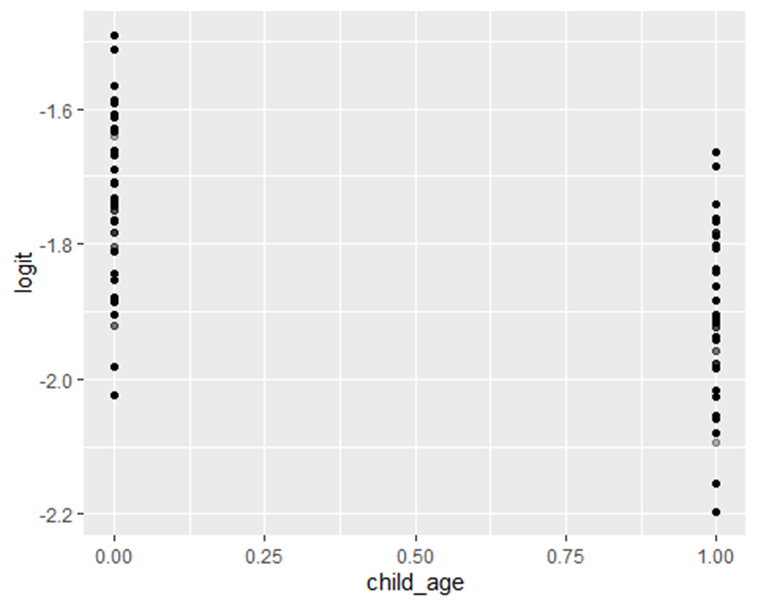
Figure 1: Distribution of full immunization by age of the child

Interactions: Interactions should be included in a model only when there is a plausible rationale based on theory or prior evidence⁸. Once included, interactions should be tested statistically and visualised to aid interpretation. In many policy-relevant analyses, certain interactions can be particularly meaningful⁴⁷; for example, the effect of education on health outcomes may differ between urban and rural residents. Careful consideration of interactions enhances the model’s ability to capture nuanced relationships and provides more actionable insights for decision-making.

R, example interaction:

mod_int <- glm(full_immunisation ~ child_age + mother_education * urban + wealth_quintile, family = binomial, data = dhs_mw)
summary(mod_int)

Call:
glm(formula = full_immunisation ~ child_age + mother_education *
    urban + wealth_quintile, family = binomial, data = dhs_mw)

Coefficients:
                                  Estimate Std. Error z value Pr(>|z|)
(Intercept)                      -1.996732   0.132556 -15.063 < 2e-16 ***
child_age                        -0.174629   0.073106 -2.389 0.01691 *
mother_educationprimary           0.008395   0.124631   0.067 0.94630
mother_educationsecondary         0.092991   0.155946   0.596 0.55097
mother_educationhigher            0.009672   0.506280   0.019 0.98476
urban1                           -0.398505   0.541564 -0.736 0.46183
wealth_quintilepoorer             0.140799   0.114704   1.227 0.21964
wealth_quintilemiddle             0.172510   0.117111   1.473 0.14074
wealth_quintilericher             0.314012   0.119719   2.623 0.00872 **
wealth_quintilerichest            0.291767   0.141237   2.066 0.03885 *
mother_educationprimary:urban1    0.547274   0.555365   0.985 0.32441
mother_educationsecondary:urban1 0.495062   0.564461   0.877 0.38046
mother_educationhigher:urban1     0.401599   0.796192   0.504 0.61398
—
Signif. codes: 0 ‘***’ 0.001 ‘**’ 0.01 ‘*’ 0.05 ‘.’ 0.1 ‘ ‘ 1

(Dispersion parameter for binomial family taken to be 1)

    Null deviance: 5132.1 on 6499 degrees of freedom
Residual deviance: 5109.4 on 6487 degrees of freedom
AIC: 5135.4

Number of Fisher Scoring iterations: 4

Random effects: When data have a hierarchical or clustered structure that is not fully accounted for by survey weights, multilevel models with random effects should be considered⁴⁸. For example, children may be nested within clusters, and clusters within districts. Multilevel models explicitly capture between-cluster variation and can provide either cluster-specific or population-averaged estimates, depending on the choice of link function and the interpretation required⁴⁹. Incorporating random effects improves model accuracy, accounts for unobserved heterogeneity, and ensures valid inference in clustered data.

R, simple multilevel example with lme4:

library(lme4)

Warning: package ‘lme4’ was built under R version 4.5.1

mod_mixed <- glmer(full_immunisation ~ child_age + mother_education + (1 | cluster), family = binomial, data = dhs_mw)
summary(mod_mixed)

Generalized linear mixed model fit by maximum likelihood (Laplace
Approximation) glmerMod
Family: binomial ( logit )
Formula: full_immunisation ~ child_age + mother_education + (1 | cluster)
   Data: dhs_mw

      AIC       BIC    logLik -2*log(L) df.resid
   4939.8    4980.4   -2463.9    4927.8      6494

Scaled residuals:
    Min      1Q Median      3Q     Max
-1.0933 -0.3682 -0.2737 -0.2371 3.9218

Random effects:
Groups Name        Variance Std.Dev.
cluster (Intercept) 1.081    1.04
Number of obs: 6500, groups: cluster, 849

Fixed effects:
                          Estimate Std. Error z value Pr(>|z|)
(Intercept)               -2.29534    0.14281 -16.072   <2e-16 ***
child_age                 -0.15959    0.07996 -1.996   0.0459 *
mother_educationprimary    0.12493    0.13413   0.931   0.3516
mother_educationsecondary 0.30202    0.15524   1.945   0.0517 .
mother_educationhigher     0.19440    0.33794   0.575   0.5651
—
Signif. codes: 0 ‘***’ 0.001 ‘**’ 0.01 ‘*’ 0.05 ‘.’ 0.1 ‘ ‘ 1

Correlation of Fixed Effects:
            (Intr) chld_g mthr_dctnp mthr_dctns
child_age   -0.284
mthr_dctnpr -0.827 0.023
mthr_dctnsc -0.732 0.009 0.759
mthr_dctnhg -0.340 0.013 0.346      0.323

Keep models parsimonious: Models should be kept as parsimonious as possible, including only predictors that are necessary and justified by theory or prior evidence. Complex models require more data to estimate parameters reliably, and overfitting can occur when too many variables are included relative to the number of outcome events. A parsimonious approach improves interpretability, reduces variance in estimates, and increases the likelihood that the model will generalise to other datasets or populations⁸.

Step 5: Model diagnostics and fit Good modelling requires checking fit and influence: Good modelling practice requires careful assessment of model fit and the influence of individual observations⁴. Multiple diagnostic tools should be employed rather than relying on a single test, as different diagnostics provide complementary information⁸. Evaluating residuals, leverage, influence measures, and overall goodness-of-fit help identify potential model misspecification, outliers, or highly influential points, ensuring that the final model is both robust and reliable.

Discrimination (AUC): Discrimination assesses a model’s ability to distinguish between individuals who experience the event and those who do not. The c-statistic, commonly referred to as the area under the receiver operating characteristic curve (AUC), provides a summary measure of this separation⁵⁰. In policy-relevant applications, an AUC above 0.7 is generally considered acceptable, while an AUC above 0.8 indicates strong discrimination; however, the interpretation should always consider the context, the outcome, and the intended use of the model⁵¹.

Calibration: Calibration evaluates whether predicted probabilities align with observed outcomes⁵². Good calibration indicates that the model’s predicted risk accurately reflects the actual probability of the event. Common approaches include calibration plots and the Hosmer-Lemeshow test⁴⁶; the Hosmer-Lemeshow test can be overly sensitive in large samples, making visual inspection of calibration curves often more informative⁴. Properly calibrated models are critical for decision-making and policy applications, ensuring that predicted risks can be interpreted with confidence⁵³.

R, Hosmer-Lemeshow, ROC, Brier:

library(ResourceSelection)

Warning: package ‘ResourceSelection’ was built under R version 4.5.1

ResourceSelection 0.3-6 2023-06-27

hoslem.test(dhs_mw$full_immunisation, fitted(mod_linear), g = 10)

Hosmer and Lemeshow goodness of fit (GOF) test

data: dhs_mw$full_immunisation, fitted(mod_linear)
X-squared = 5.644, df = 8, p-value = 0.687

library(pROC)

Type ‘citation(“pROC”)’ for a citation.

Attaching package: ‘pROC’

The following objects are masked from ‘package:stats’:

cov, smooth, var

roc_obj <- roc(dhs_mw$full_immunisation, fitted(mod_linear))

Setting levels: control = 0, case = 1

Setting direction: controls < cases

auc(roc_obj)

Area under the curve: 0.5484

# Brier score
mean((dhs_mw$full_immunisation – fitted(mod_linear))^2)

1 0.1159879

Residuals and influential points: Assessing residuals and influential points is essential to ensure model robustness⁴. Evaluating residuals, leverage, and influence measures helps identify observations that may disproportionately affect coefficient estimates⁵⁵. This is particularly important in small samples, where single extreme or influential observations can distort results. Detecting and addressing such points through careful investigation or sensitivity analyses improves model reliability and strengthens confidence in the findings.

infl <- influence.measures(mod_linear)
#summary(infl) #Activate this to see the results

Model validation: Model validation is a critical step in both predictive and inferential analyses⁵⁷. For prediction-focused models, internal validation can be performed using cross-validation or hold-out samples to assess performance and generalisability⁵⁸. For inference-oriented models, bootstrapping provides a way to evaluate optimism, adjust confidence intervals, and check the stability of parameter estimates. In practice, tools such as the caret⁵⁹ or cv.glmnet⁶⁰ packages in R facilitate cross-validation for penalised models⁶¹, while the rms⁶² package supports bootstrapping for inferential models. It is essential to report validation diagnostics in the manuscript, include relevant plots in supplementary materials, and document any influential observations that were removed or retained, ensuring transparency and reproducibility.

Step 6: Interpretation and presentation

Interpreting model results in a clear and actionable way is essential⁶³, especially for policy and decision-making. While odds ratios are standard outputs in logistic regression, they can be difficult to interpret when the outcome is common⁶⁴. Whenever possible, presenting predicted probabilities, absolute risks, or risk differences provides a more intuitive understanding of the effect sizes and facilitates practical decision-making⁶⁵. Translating statistical findings into measures that are directly meaningful to stakeholders enhances the usability and impact of the research.

Odds ratios and confidence intervals, R:

library(broom)
tidy(mod_linear, exponentiate = TRUE, conf.int = TRUE)

# A tibble: 10 × 7
   term                 estimate std.error statistic p.value conf.low conf.high
   <chr>                   <dbl>     <dbl>     <dbl>    <dbl>    <dbl>     <dbl>
1 (Intercept)             0.132    0.131    -15.5   6.11e-54    0.102     0.170
2 child_age               0.841    0.0731    -2.38 1.75e- 2    0.728     0.970
3 mother_educationpri…    1.04     0.121      0.344 7.31e- 1    0.826     1.33
4 mother_educationsec…    1.12     0.145      0.809 4.18e- 1    0.848     1.50
5 mother_educationhig…    0.967    0.308     -0.108 9.14e- 1    0.515     1.73
6 wealth_quintilepoor…    1.15     0.115      1.20 2.30e- 1    0.917     1.44
7 wealth_quintilemidd…    1.19     0.117      1.46 1.45e- 1    0.943     1.49
8 wealth_quintilerich…    1.37     0.119      2.63 8.55e- 3    1.08      1.73
9 wealth_quintilerich…    1.34     0.141      2.07 3.85e- 2   1.01      1.76
10 urban1                  1.11     0.114      0.892 3.72e- 1    0.884     1.38

Predicted probabilities and marginal effects, R:

newdata <- expand.grid(child_age = c(1, 2), mother_education = c(“none”,”secondary”),
wealth_quintile = c(“poorest”,”richest”), urban = c(0,1))

newdata$urban <- factor(newdata$urban, levels = levels(dhs_mw$urban))

newdata$pred <- predict(mod_linear, newdata, type = “response”)
newdata

   child_age mother_education wealth_quintile urban      pred
1          1             none         poorest     0 0.10006454
2          2             none         poorest     0 0.08547725
3          1        secondary         poorest     0 0.11117341
4          2        secondary         poorest     0 0.09513788
5          1             none         richest     0 0.12958323
6          2             none         richest     0 0.11122458
7          1        secondary         richest     0 0.14344683
8          2        secondary         richest     0 0.12340252
9          1             none         poorest     1 0.10959612
10         2             none         poorest     1 0.09376410
11         1        secondary         poorest     1 0.12162015
12         2        secondary         poorest     1 0.10425454
13         1             none         richest     1 0.14148453
14         2             none         richest     1 0.12167547
15         1        secondary         richest     1 0.15639262
16         2        secondary         richest     1 0.13482409

Common outcomes: When the outcome of interest is common, odds ratios can overstate the magnitude of associations, making interpretation challenging. In such cases, reporting adjusted risk ratios can provide a more intuitive measure of effect⁶⁷. A practical approach is to use a Poisson regression model with robust standard errors⁴, which yields approximate risk ratios that are easier for policymakers and other stakeholders to interpret and act upon. This method improves the clarity and usability of findings without compromising statistical validity.

R, Poisson with robust SE:

library(sandwich)
library(lmtest)

Loading required package: zoo

Attaching package: ‘zoo’

The following objects are masked from ‘package:base’:

as.Date, as.Date.numeric

mod_pois <- glm(full_immunisation ~ child_age + mother_education + wealth_quintile + urban,
family = poisson(link = “log”), data = dhs_mw)
coeftest(mod_pois, vcov = vcovHC(mod_pois, type = “HC0”))

z test of coefficients:

                           Estimate Std. Error z value Pr(>|z|)
(Intercept)               -2.148666   0.117840 -18.2337 < 2.2e-16 ***
child_age                 -0.149931   0.063185 -2.3729 0.017649 *
mother_educationprimary    0.036564   0.105423   0.3468 0.728720
mother_educationsecondary 0.101486   0.125990   0.8055 0.420525
mother_educationhigher    -0.026540   0.263740 -0.1006 0.919846
wealth_quintilepoorer      0.120942   0.100385   1.2048 0.228285
wealth_quintilemiddle      0.149702   0.101941   1.4685 0.141963
wealth_quintilericher      0.271568   0.102762   2.6427 0.008225 **
wealth_quintilerichest     0.253477   0.121070   2.0936 0.036292 *
urban1                     0.086229   0.094482   0.9126 0.361428
—
Signif. codes: 0 ‘***’ 0.001 ‘**’ 0.01 ‘*’ 0.05 ‘.’ 0.1 ‘ ‘ 1

Tables and figures: Effective presentation of results is critical for clarity and impact. Tables should clearly display adjusted estimates, sample sizes, number of events, and key model fit statistics⁶⁸. Supplementary tables can provide a complete list of variables considered, along with the code used to generate the final model, supporting transparency and reproducibility. Visualisations, such as predicted probability plots, are particularly valuable for communicating results to policymakers, translating complex statistical outputs into intuitive insights that can inform decision-making⁶⁹.

Language and claims: When reporting results from observational studies, careful attention should be paid to the language used⁷⁰. Causal claims should be avoided unless the study design and methods explicitly support them⁷¹. Instead of stating that “X causes Y,” it is more appropriate to describe findings as “X is associated with Y.” For prediction-focused analyses, terms such as “predicts” or “forecast” are suitable, reflecting the model’s purpose without implying causation. Using cautious and precise language enhances credibility and prevents overinterpretation of the results¹⁷.

Practical checklist to finish modelling

Before you write results, tick these items:

Outcome coded and documented, 0/1, event defined: Outcomes should be coded consistently as 0 and 1, with the event clearly defined. All recoding steps must be documented to ensure transparency and reproducibility.
Missing data handled, and method reported: Patterns of missing data should be explored, appropriate methods applied, and the chosen approach clearly reported. Multiple imputation is often preferred over complete-case analysis when missingness is substantial.
Survey design accounted for when needed: When working with complex survey data, stratification, clustering, and weights should be accounted for using survey-aware methods to produce valid estimates and standard errors.
EPV checked, penalisation used if EPV is low: The ratio of outcome events to predictors should be checked. If EPV is low, the number of predictors can be reduced, categories collapsed, or penalised methods such as lasso or Firth regression applied.
Linearity in logit assessed, non-linear terms used when needed: Continuous predictors should be assessed for linearity in the logit. Non-linear relationships can be accommodated using splines or fractional polynomials to improve model fit.
Interactions tested only when sensible: Interactions should only be included when there is a plausible rationale. Testing and visualising interactions aids interpretation, such as examining how effects differ by subgroups like urban versus rural residents.
Diagnostics run, AUC and calibration reported, influential points checked: Model diagnostics should be conducted thoroughly. Report discrimination (AUC), calibration, residuals, and check for influential points to ensure model robustness.
Results presented with ORs or RRs, predicted probabilities and clear interpretation: Present results with interpretable measures such as odds ratios, risk ratios, predicted probabilities, or risk differences. Clear presentation helps stakeholders and policymakers understand and act on findings.
Code and data workflow saved for reproducibility: All code, workflows, and key decisions should be saved and documented to allow others to replicate the analysis and verify results.

Common pitfalls and how to avoid them

Despite its power and flexibility, logistic regression is often misapplied in clinical and public health research. These errors can weaken the validity of findings, obscure important associations, and sometimes lead to misleading policy recommendations⁴³. Below, we outline frequent pitfalls, illustrate them with examples from global and African contexts, and provide practical strategies to avoid them; complete with R code snippets for immediate use. By recognizing these common pitfalls and applying these practical solutions, health researchers can ensure their logistic regression analyses are robust, interpretable, and useful for decision-making. This is especially critical in settings where data and analytical challenges are common.

Misunderstanding the Odds Ratio Odds ratios can overstate the magnitude of associations when outcomes are common, typically above 10%⁷³. For instance, in Malawi, facility delivery rates are often high, so ORs may exaggerate the perceived effect. To avoid misinterpretation, it is advisable to report marginal effects, predicted probabilities, or adjusted risk ratios alongside ORs, and to provide clear explanations of what each measure represents.

# Display odds ratios with confidence intervals
library(broom)
mod_logistic = mod_int
tidy(mod_logistic, exponentiate = TRUE, conf.int = TRUE)

# A tibble: 13 × 7
   term                 estimate std.error statistic p.value conf.low conf.high
   <chr>                   <dbl>     <dbl>     <dbl>    <dbl>    <dbl>     <dbl>
1 (Intercept)             0.136    0.133   -15.1    2.82e-51    0.104     0.175
2 child_age               0.840    0.0731   -2.39   1.69e- 2    0.727     0.969
3 mother_educationpri…    1.01     0.125     0.0674 9.46e- 1    0.794     1.29
4 mother_educationsec…    1.10     0.156     0.596 5.51e- 1    0.809     1.49
5 mother_educationhig…    1.01     0.506     0.0191 9.85e- 1    0.332     2.52
6 urban1                  0.671    0.542    -0.736 4.62e- 1    0.197     1.74
7 wealth_quintilepoor…    1.15     0.115     1.23   2.20e- 1    0.919     1.44
8 wealth_quintilemidd…    1.19     0.117     1.47   1.41e- 1    0.944     1.50
9 wealth_quintilerich…    1.37     0.120     2.62   8.72e- 3    1.08      1.73
10 wealth_quintilerich…    1.34     0.141     2.07   3.88e- 2    1.01      1.76
11 mother_educationpri…    1.73     0.555     0.985 3.24e- 1    0.646     6.02
12 mother_educationsec…    1.64     0.564     0.877 3.80e- 1    0.600     5.79
13 mother_educationhig…    1.49     0.796     0.504 6.14e- 1    0.338     7.98

# Calculate predicted probabilities (marginal effects)
newdata <- data.frame(
mother_education = c(“none”, “primary”),
urban = c(0, 1),
wealth_quintile = c(“richest”, “middle”),
child_age = c(1, 1)
)
newdata$urban <- factor(newdata$urban, levels = levels(dhs_mw$urban))

newdata$pred_prob <- predict(mod_logistic, newdata, type = “response”)
print(newdata)

mother_education urban wealth_quintile child_age pred_prob
1 none 0 richest 1 0.1324355
2 primary 1 middle 1 0.1368518

Ignoring linearity in the logit for continuous predictors Failing to check whether continuous variables have a linear relationship with the log odds can lead to biased coefficient estimates and misinterpretation⁷⁴. To address this, the relationship should be assessed using graphical methods, and non-linear terms such as splines or fractional polynomials can be incorporated when needed.

# library(splines)
# dhs_mw$mother_age <- as.numeric(dhs_mw$mother_age)
# mod_linear <- glm(full_immunisation ~ mother_age + child_age, family = binomial, data = dhs_mw)
# mod_spline <- glm(full_immunisation ~ ns(mother_age, df = 4) + child_age, family = binomial, data = dhs_mw)
# anova(mod_linear, mod_spline, test = “Chisq”)

Overfitting the model Including too many predictors relative to the number of outcome events can produce unstable estimates and reduce generalisability. To avoid overfitting, maintain at least 10 EPV, or, when this is not possible, use penalised regression methods such as lasso, ridge, or Firth logistic regression⁷⁶.

# # Calculate EPV
# events <- sum(df$outcome == 1)
# num_predictors <- length(coef(mod_logistic)) – 1
# epv <- events / num_predictors
# print(epv)
#
# # Example of penalised logistic regression with LASSO
# library(glmnet)
# x <- model.matrix(outcome ~ ., df),-1
# y <- df$outcome
# cvfit <- cv.glmnet(x, y, family = “binomial”, alpha = 1)
# coef(cvfit, s = “lambda.min”)

Omitted variable bias Failing to include important confounders can produce biased estimates of effects and mislead conclusions. To avoid this, predictors should be selected based on domain knowledge, prior literature, or formal tools such as directed acyclic graphs (DAGs) to identify key confounding variables⁷⁸.

No direct code, but ensure confounders are in your model syntax, e.g.: glm(outcome ~ exposure + confounder1 + confounder2, family = binomial, data = df)

Multicollinearity Highly correlated predictors can inflate standard errors and destabilise coefficient estimates, reducing model reliability. To address multicollinearity, variance inflation factors (VIF) should be checked, and highly correlated variables can be removed, combined, or otherwise reduced through dimensionality reduction techniques.

library(car)
vif(mod_logistic)

there are higher-order terms (interactions) in this model
consider setting type = ‘predictor’; see ?vif

                             GVIF Df GVIF^(1/(2*Df))
child_age                1.003608 1        1.001802
mother_education         5.600133 3        1.332600
urban                   32.683686 1        5.716965
wealth_quintile          1.737765 4        1.071517
mother_education:urban 140.361228 3        2.279683

Complete or quasi-complete separation When a predictor perfectly or nearly perfectly predicts the outcome, standard logistic regression cannot estimate coefficients reliably, leading to model failure. To address this, penalised regression methods such as Firth’s logistic regression can be used, providing stable estimates even in the presence of separation⁸¹.

# # Firth logistic regression using logistf package
# library(logistf)
#
# newdata$full_immunisation <- c(1, 0) # Add the outcomes
#
# firth_mod <- logistf(full_immunisation ~ mother_education + wealth_quintile + urban + child_age, data = newdata)
# summary(firth_mod)

Ignoring interaction effects Failing to include meaningful interactions can conceal important differences in how predictors affect the outcome across subgroups⁸³. To address this, interactions should be tested and included when supported by theory or prior evidence, and results should be visualised to aid interpretation.

# mod_interaction <- glm(outcome ~ predictor1 * predictor2 + other_vars, family = binomial, data = df)
# summary(mod_interaction)

Poor Handling of missing data

Relying solely on complete-case analysis can produce biased results when data are not missing completely at random⁸⁵. To avoid this, patterns of missingness should be explored, and appropriate methods such as multiple imputation⁸⁶ should be applied to reduce bias and maintain statistical power.

# library(mice)
# md.pattern(dhs_mw)
# imp <- mice(df, m = 5, method = ‘pmm’, seed = 123)
# fit_imp <- with(imp, glm(outcome ~ predictors, family = binomial))
# pool(fit_imp)

Inadequate model diagnostics

Failing to assess model fit and predictive performance can lead to misleading conclusions⁸⁷. To avoid this, a combination of diagnostics should be used, including the Hosmer–Lemeshow test, ROC/AUC for discrimination, calibration plots, and checks of residuals and influential points, ensuring the model is robust and reliable.

library(ResourceSelection)
hoslem.test(dhs_mw$full_immunisation, fitted(mod_logistic), g = 10)

Hosmer and Lemeshow goodness of fit (GOF) test

data: dhs_mw$full_immunisation, fitted(mod_logistic)
X-squared = 4.4301, df = 8, p-value = 0.8164

library(pROC)
roc_obj <- roc(dhs_mw$full_immunisation, fitted(mod_logistic))

Setting levels: control = 0, case = 1

Setting direction: controls < cases

auc(roc_obj)

Area under the curve: 0.5488

plot(roc_obj)

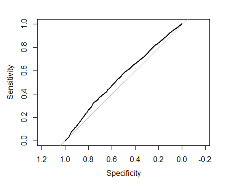
Figure 2: Sensitivity and specificity of the fitted model

Over-reliance on P-values

Focusing solely on statistical significance can obscure the practical importance of findings⁸⁸. To avoid this, effect sizes and confidence intervals should be reported alongside p-values, and the discussion should emphasise real-world relevance and policy implications.

No code needed but ensure your results tables include estimates with 95% confidence intervals and interpret them clearly.

Policy and Practice relevance: Logistic regression in clinical and public health research is not an end in itself. The ultimate goal is to inform policies and interventions that improve health outcomes⁸⁹. This section highlights how to interpret, communicate, and apply logistic regression findings to support evidence-based decision-making⁹⁰, with examples from African and global health contexts.

From Odds Ratios to Meaningful Measures

While odds ratios are standard outputs in logistic regression, they can be abstract and unintuitive, especially for non-technical audiences. Expressing results as predicted probabilities, absolute risks, or risk differences provides a clearer, more actionable view of the findings, making it easier for policymakers to understand and use the information for decision-making⁹¹. Example: In Malawi’s DHS analysis on childhood immunisation, an OR of 2.5 for maternal secondary education might sound large. But translating this into a predicted probability increase (e.g., from 60% to 85% immunisation coverage) better illustrates the potential impact of education-focused programs.

R code to calculate and plot predicted probabilities:

library(ggplot2)
# Create new data for different maternal education levels
newdata <- data.frame(
mother_education = factor(c(“none”, “primary”, “secondary”, “higher”),
                           levels = c(“none”, “primary”, “secondary”, “higher”)),
child_age = mean(dhs_mw$child_age, na.rm = TRUE),
wealth_quintile = “middle”,
urban = 0
)

# Match the factor structure of the model
newdata$urban <- factor(newdata$urban, levels = levels(dhs_mw$urban))

# Predict probabilities
newdata$pred_prob <- predict(mod_logistic, newdata, type = “response”)

# Plot predicted probabilities with 95% CI
ggplot(newdata, aes(x = mother_education, y = pred_prob)) +
geom_point(size = 3) +
ylim(0,1) +
labs(title = “Predicted Probability of Full Immunisation by Maternal Education”,
       x = “Maternal Education Level”,
       y = “Predicted Probability”) +
theme_minimal()

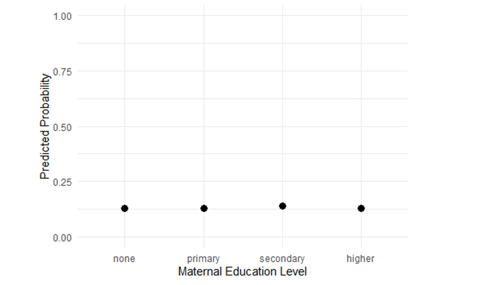
Figure 3: Probability of full immunisation by

Identifying high-risk groups for targeted interventions Logistic regression is a valuable tool for identifying populations at higher risk of adverse outcomes⁹². By highlighting groups with elevated predicted probabilities, it helps policymakers and program managers target interventions more effectively, ensuring that resources are directed where they are most needed⁹³. Example: In Malawi DHS data (2004-2016), logistic regression revealed informal employment, being male, and low education significantly reduce the odds of HIV testing uptake⁹⁴. Such evidence supports outreach campaigns in rural areas targeting low-education groups.

R code snippet to generate subgroup predicted probabilities:

# Define groups for prediction
newdata <- expand.grid(
urban = c(0, 1),
mother_education = factor(c(“none”, “secondary”), levels = levels(dhs_mw$mother_education)),
child_age = mean(dhs_mw$child_age, na.rm = TRUE),
wealth_quintile = “middle”
)

# Match the factor structure of the model
newdata$urban <- factor(newdata$urban, levels = levels(dhs_mw$urban))

newdata$pred_prob <- predict(mod_logistic, newdata, type = “response”)
print(newdata)

urban mother_education child_age wealth_quintile pred_prob
1     0             none 0.5003077          middle 0.12880232
2     1             none 0.5003077          middle 0.09029033
3     0        secondary 0.5003077          middle 0.13960206
4     1        secondary 0.5003077          middle 0.15160838

Informing resource allocation

Quantifying how predictors influence predicted probabilities can directly inform resource allocation. For example, if wealth quintile strongly affects hypertension treatment in Zambia⁹⁵, programs can target support to lower-income groups. Policymakers often prefer absolute differences in risk or predicted probabilities rather than odds ratios, as these measures clearly indicate the potential impact of interventions and facilitate practical decision-making.

R code to calculate risk differences:

library(margins)

Warning: package ‘margins’ was built under R version 4.5.1

mod_logistic <- glm(full_immunisation ~ wealth_quintile + child_age + wealth_quintile, family = binomial, data = dhs_mw)

# Calculate marginal effects (risk differences)
marg_eff <- margins(mod_logistic)
summary(marg_eff)

factor AME SE z p lower upper
child_age -0.0202 0.0085 -2.3872 0.0170 -0.0368 -0.0036
wealth_quintilemiddle 0.0197 0.0125 1.5784 0.1145 -0.0048 0.0442
wealth_quintilepoorer 0.0153 0.0120 1.2725 0.2032 -0.0083 0.0389
wealth_quintilericher 0.0394 0.0133 2.9552 0.0031 0.0133 0.0655
wealth_quintilerichest 0.0442 0.0135 3.2746 0.0011 0.0177 0.0706

Presenting results to non-technical audiences

Clear visualisation and simple language improve uptake of findings.

Use predicted probability plots rather than tables of ORs alone.
Translate statistics into plain English: e.g., “Children of mothers with secondary education are 25 percentage points more likely to be fully immunised.”
Highlight policy-relevant variables.
Discuss limitations and uncertainties openly.
Supporting program evaluation and monitoring Repeated logistic regression analyses on program data can help track progress over time, identify barriers to implementation, and inform mid-course corrections⁴². By quantifying changes in predicted probabilities or risk differences, programs can evaluate effectiveness and adjust strategies to better reach high-risk populations⁹⁶. Example: In a malaria control program in Nigeria, logistic regression showed bed net ownership strongly predicted prevention behavior. Over time, logistic regression helped evaluate if increased net distribution translated into behavior change.

Cautions in Policy and Application:

Associations do not equal causation: Logistic regression applied to observational data identifies associations and potential targets, but it does not establish causal relationships8. Findings should be interpreted cautiously, and causal claims should only be made if supported by study design or additional evidence. Clear language helps prevent misinterpretation and overstatement of results⁹⁷.
Consider confounding and bias: When interpreting regression results for policy decisions, it is essential to account for potential confounding and other sources of bias⁹⁸. Associations observed in the data may be influenced by unmeasured or inadequately controlled factors, and failing to consider these can lead to inappropriate recommendations⁹⁷. Careful model specification, adjustment for key confounders, and transparent reporting strengthen the reliability of findings for decision-making.
Community engagement: Logistic regression provides valuable quantitative evidence, but combining these results with qualitative insights and community engagement enriches interpretation⁹⁹. Local and expert knowledge can contextualise statistical associations, highlight barriers or enablers not captured in the data, and guide the design of interventions that are culturally appropriate and feasible, ensuring that policies are both evidence- and expert-informed and locally relevant¹⁰⁰.

Conclusion and Recommendations

Logistic regression remains a fundamental tool in clinical and public health research, offering insights into factors associated with key health outcomes. Logistic regression results become truly valuable when translated into understandable, actionable insights. Using predicted probabilities, risk differences, and subgroup analyses helps policymakers prioritise interventions, allocate resources efficiently, and communicate findings effectively. Including clear visualisations and plain-language interpretations enhances impact in global and African health settings. When applied carefully, it can guide policy and practice across diverse settings, including complex health systems. This paper has presented a practical guide to the core considerations in logistic regression modelling. We highlighted essential steps from defining clear research questions, preparing data thoughtfully, choosing variables wisely, specifying models correctly, to conducting thorough diagnostics. Common pitfalls such as overfitting, misinterpreting odds ratios, ignoring interactions, and mishandling missing data were identified, alongside concrete ways to avoid them. Finally, we emphasized translating statistical results into meaningful, actionable evidence for policymakers and practitioners.

Key recommendations for researchers and practitioners include:

Plan carefully from the start: Define your outcome clearly, understand your data’s limitations, and anticipate sample size needs to ensure robust models.
Prepare and code variables thoughtfully: Treat continuous predictors properly, handle missing data with modern methods like multiple imputation, and account for survey design complexities.
Use variable selection strategies that balance theory and data-driven approaches: Avoid automatic stepwise selection without validation.
Check model assumptions rigorously: Evaluate linearity, interactions, collinearity, and separation issues; adjust models accordingly.
Validate your models: Use internal validation techniques such as bootstrapping or cross-validation to assess reliability and generalizability.
Present results clearly and meaningfully: Go beyond odds ratios—provide predicted probabilities, risk differences, and subgroup analyses to inform practical decisions.
Communicate findings in plain language with supportive visuals: This enhances uptake by non-technical audiences including policymakers, program managers, and communities.
Recognize the limits of observational data: Use logistic regression results as one part of evidence, integrating other study designs and community perspectives.

By following these principles, global and African public health researchers can harness logistic regression to generate credible, actionable evidence. This evidence can support the design, targeting, and evaluation of interventions that improve health outcomes and reduce inequities.

Funding

None

Competing interests

We declare no competing interests.

Availability of data

All data are available within the manuscript.

Author contributions

WFN= Conceptualization and drafting the paper and code. CZ and ASM=Reviewing the paper and the code. Both authors reviewed and approved the paper together with the code.

References

1. Schober, P., & Vetter, T. R. (2021). Logistic regression in medical research. Anesthesia and Analgesia, 132(2), 365–366. https://doi.org/10.1213/ANE.0000000000005247
2. Gallis, J. A., & Turner, E. L. (2019). Relative measures of association for binary outcomes: Challenges and recommendations for the global health researcher. Annals of Global Health, 85(1), 137. https://doi.org/10.5334/aogh.2581
3. Vittinghoff, E., Glidden, D. V., Shiboski, S. C., & McCulloch, C. E. (2012). Regression methods in biostatistics: Linear, logistic, survival, and repeated measures models. Springer. https://doi.org/10.1007/978-1-4614-1353-0
4. Hilbe, J. M. (2009). Logistic regression models (1st ed.). Chapman & Hall.
5. Pearce, N. (2016). Analysis of matched case-control studies. BMJ (Clinical Research Ed.), 352, i969. https://doi.org/10.1136/bmj.i969
6. Rothman, K. J. (2008). Epidemiology: An introduction (2nd ed.). Oxford University Press.
7. Vandenbroucke, J. P., & Pearce, N. (2007). Case-control studies: Basic concepts. International Journal of Epidemiology, 36(5), 948–952. https://doi.org/10.1093/ije/dym207
8. Harrell, F. E. (2015). Regression modeling strategies: With applications to linear models, logistic and ordinal regression, and survival analysis. Springer Series in Statistics, 39. https://doi.org/10.1007/978-3-319-19425-7
10. Franzen, S. R., Chandler, C., & Lang, T. (2017). Health research capacity development in low and middle income countries: Reality or rhetoric? A systematic meta-narrative review of the qualitative literature. BMJ Open, 7(1), e012332. https://doi.org/10.1136/bmjopen-2016-012332
11. Sheffel, A., Wilson, E., Munos, M., & Zeger, S. (2019). Methods for analysis of complex survey data: An application using the tanzanian 2015 demographic and health survey and service provision assessment. Journal of Global Health, 9(2), 020902. https://doi.org/10.7189/jogh.09.020902
12. Simundić, A.-M. (2013). Bias in research. Biochemia Medica (Zagreb), 23(1), 12–15. https://doi.org/10.11613/bm.2013.003
13. Faber, J., & Fonseca, L. M. (2014). How sample size influences research outcomes. Dental Press Journal of Orthodontics, 19(4), 27–29. https://doi.org/10.1590/2176-9451.19.4.027-029.ebo
14. Carpenter, J. R., & Smuk, M. (2021). Missing data: A statistical framework for practice. Biometrical Journal, 63(5), 915–947. https://doi.org/10.1002/bimj.202000196
15. Ozgur, C., Kleckner, M., & Li, Y. (2015). Selection of statistical software for solving big data problems: A guide for businesses, students, and universities. SAGE Open, 5(2). https://doi.org/10.1177/2158244015584379
16. Shrier, I., Redelmeier, D. A., Schnitzer, M. E., & Steele, R. J. (2021). Challenges in interpreting results from ’multiple regression’ when there is interaction between covariates. BMJ Evidence-Based Medicine, 26(2), 53–56. https://doi.org/10.1136/bmjebm-2019-111225
17. Ito, C., Al-Hassany, L., Kurth, T., & Glatz, T. (2025). Distinguishing description, prediction, and causal inference: A primer on improving congruence between research questions and methods. Neurology, 104(4), e210171. https://doi.org/10.1212/WNL.0000000000210171
18. Ratan, S. K., Anand, T., & Ratan, J. (2019). Formulation of research question – stepwise approach. Journal of Indian Association of Pediatric Surgeons, 24(1), 15–20. https://doi.org/10.4103/jiaps.JIAPS_76_18
19. Hammerton, G., & Munafò, M. R. (2021). Causal inference with observational data: The need for triangulation of evidence. Psychological Medicine, 51(4), 563–578. https://doi.org/10.1017/S0033291720005127
20. Elshawi, R., Al-Mallah, M. H., & Sakr, S. (2019). On the interpretability of machine learning-based model for predicting hypertension. BMC Medical Informatics and Decision Making, 19, 146. https://doi.org/10.1186/s12911-019-0874-0
21. Heinze, G., Wallisch, C., & Dunkler, D. (2018). Variable selection – a review and recommendations for the practicing statistician. Biometrical Journal, 60(3), 431–449. https://doi.org/10.1002/bimj.201700067
22. Iacobucci, D., Schneider, M. J., Popovich, D. L., & Bakamitsos, G. A. (2016). Mean centering helps alleviate “micro” but not “macro” multicollinearity. Behavior Research Methods, 48, 1308–1317. https://doi.org/10.3758/s13428-015-0624-x
23. Dong, Y., & Peng, C. J. (2013). Principled missing data methods for researchers. SpringerPlus, 2(1), 222. https://doi.org/10.1186/2193-1801-2-222
24. Sterne, J. A. C., White, I. R., Carlin, J. B., Spratt, M., Royston, P., Kenward, M. G., Wood, A. M., & Carpenter, J. R. (2009). Multiple imputation for missing data in epidemiological and clinical research: Potential and pitfalls. BMJ, 338, b2393. https://doi.org/10.1136/bmj.b2393
25. Buuren, S. van. (2018). Flexible imputation of missing data (2nd ed.). Chapman & Hall/CRC.
26. Ross, R., Breskin, A., & Westreich, D. (2020). When is a complete case approach to missing data valid? The importance of effect measure modification. American Journal of Epidemiology, 189. https://doi.org/10.1093/aje/kwaa124
27. Szwarcwald, C. L. (2023). National health surveys: Overview of sampling techniques and data collected using complex designs. Epidemiologia e Serviços de Saúde, 32(3), e2023431. https://doi.org/10.1590/S2237-96222023000300014.EN
28. Lumley, T., Diehr, P., Emerson, S., & Chen, L.-J. (2004). The importance of the normality assumption in large public health data sets. Annual Review of Public Health, 25(1), 151–169. https://doi.org/10.1146/annurev.publhealth.25.101802.123014
29. Heeringa, S. G., West, B. T., & Berglund, P. A. (2017). Applied survey data analysis. Chapman and Hall/CRC. https://doi.org/10.1201/9781315371650
30. Lumley, T. (2011). Complex surveys: A guide to analysis using r. Wiley. https://doi.org/10.1002/9781118257607
31. Choi, G., Buckley, J. P., Kuiper, J. R., & Keil, A. P. (2022). Log-transformation of independent variables: Must we? Epidemiology, 33(6), 843–853. https://doi.org/10.1097/EDE.0000000000001534
32. Kwak, S. K., & Kim, J. H. (2017). Statistical data preparation: Management of missing values and outliers. Korean Journal of Anesthesiology, 70(4), 407–411. https://doi.org/10.4097/kjae.2017.70.4.407
34. Piccininni, M., Konigorski, S., Rohmann, J. L., & Kurth, T. (2020). Directed acyclic graphs and causal thinking in clinical risk prediction modeling. BMC Medical Research Methodology, 20(1), 179. https://doi.org/10.1186/s12874-020-01058-z
35. Pearl, J. (2009). Causal inference in statistics: An overview. Statistics Surveys, 3, 96–146. https://doi.org/10.1214/09-SS057
36. Dyer, B. P. (2025). Variable selection for causal inference, prediction, and descriptive research: A narrative review of recommendations. European Heart Journal Open, 5(3), oeaf070. https://doi.org/10.1093/ehjopen/oeaf070
37. Westreich, D., & Greenland, S. (2013). The table 2 fallacy: Presenting and interpreting confounder and modifier coefficients. American Journal of Epidemiology, 177(4), 292–298. https://doi.org/10.1093/aje/kws412
38. Bujang, M. A., Sa’at, N., Sidik, T., & Joo, L. C. (2018). Sample size guidelines for logistic regression from observational studies with large population: Emphasis on the accuracy between statistics and parameters based on real life clinical data. Malaysian Journal of Medical Sciences, 25(4), 122–130. https://doi.org/10.21315/mjms2018.25.4.12
39. Altelbany, S. (2021). Evaluation of ridge, elastic net and lasso regression methods in precedence of multicollinearity problem: A simulation study. Journal of Applied Economics and Business Studies, 5, 131–142. https://doi.org/10.34260/jaebs.517
40. James, G., Witten, D., Hastie, T., & Tibshirani, R. (2013). An introduction to statistical learning (Vol. 112, pp. 3–7). Springer. https://doi.org/10.1007/978-1-4614-7138-7
41. Vatcheva, K. P., Lee, M., McCormick, J. B., & Rahbar, M. H. (2016). Multicollinearity in regression analyses conducted in epidemiologic studies. Epidemiology (Sunnyvale), 6(2), 227. https://doi.org/10.4172/2161-1165.1000227
42. Kirkwood, B. R., & Sterne, J. A. C. (2003). Essential medical statistics. Blackwell Science.
43. Ranganathan, P., Pramesh, C. S., & Aggarwal, R. (2017). Common pitfalls in statistical analysis: Logistic regression. Perspectives in Clinical Research, 8(3), 148–151. https://doi.org/10.4103/picr.PICR_87_17
45. Schuster, N. A., Rijnhart, J. J. M., Twisk, J. W. R., & Heymans, M. W. (2022). Modeling non-linear relationships in epidemiological data: The application and interpretation of spline models. Frontiers in Epidemiology, 2, 975380. https://doi.org/10.3389/fepid.2022.975380
46. Hosmer, D. W., Lemeshow, S., & Sturdivant, R. X. (2013). Applied logistic regression. Wiley Series in Probability and Statistics, 398. https://doi.org/10.1002/9781118548387
47. Cotter, J., Schmiege, S., Moss, A., & Ambroggio, L. (2023). How to interact with interactions: What clinicians should know about statistical interactions. Hospital Pediatrics, 13(10), e319–e323. https://doi.org/10.1542/hpeds.2023-007259
48. Bender, R., Augustin, T., & Blettner, M. (2005). Generalisability and the random effects model. Biometrical Journal, 47(1), 19–31. https://doi.org/10.1002/bimj.200410258
49. Austin, P. C., Kapral, M. K., Vyas, M. V., Fang, J., & Yu, A. Y. X. (2024). Using multilevel models and generalized estimating equation models to account for clustering in neurology clinical research. Neurology, 103(9), e209947. https://doi.org/10.1212/WNL.0000000000209947
50. Sadatsafavi, M., Saha-Chaudhuri, P., & Petkau, J. (2022). Model-based ROC curve: Examining the effect of case mix and model calibration on the ROC plot. Medical Decision Making, 42(4), 487–499. https://doi.org/10.1177/0272989X211050909
51. Çorbacıoğlu, Ş. K., & Aksel, G. (2023). Receiver operating characteristic curve analysis in diagnostic accuracy studies: A guide to interpreting the area under the curve value. Turkish Journal of Emergency Medicine, 23(4), 195–198. https://doi.org/10.4103/tjem.tjem_182_23
52. Walsh, C., Sharman, K., & Hripcsak, G. (2017). Beyond discrimination: A comparison of calibration methods and clinical usefulness of predictive models of readmission risk. Journal of Biomedical Informatics, 76, 10.1016/j.jbi.2017.10.008. https://doi.org/10.1016/j.jbi.2017.10.008
53. Huang, Y., Li, W., Macheret, F., Gabriel, R. A., & Ohno-Machado, L. (2020). A tutorial on calibration measurements and calibration models for clinical prediction models. Journal of the American Medical Informatics Association, 27(4), 621–633. https://doi.org/10.1093/jamia/ocz228
54. Zhang, Z. (2016). Residuals and regression diagnostics: Focusing on logistic regression. Annals of Translational Medicine, 4(10), 195. https://doi.org/10.21037/atm.2016.03.36
55. Dey, D., Haque, M. S., Islam, M. M., et al. (2025). The proper application of logistic regression model in complex survey data: A systematic review. BMC Medical Research Methodology, 25, 15. https://doi.org/10.1186/s12874-024-02454-5
56. Steyerberg, E. W. (2010). Clinical prediction models: A practical approach to development, validation, and updating. Springer. https://doi.org/10.1007/978-0-387-77244-8
57. Shmueli, G. (2010). To explain or to predict? Statistical Science, 25(3), 289–310. https://doi.org/10.1214/10-STS330
58. Coley, R. Y., Liao, Q., Simon, N., & Shortreed, S. M. (2023). Empirical evaluation of internal validation methods for prediction in large-scale clinical data with rare-event outcomes: A case study in suicide risk prediction. BMC Medical Research Methodology, 23(1), 33. https://doi.org/10.1186/s12874-023-01844-5
59. Kuhn, M. (2008). Building predictive models in r using the caret package. Journal of Statistical Software, 28, 1–26. https://doi.org/10.18637/jss.v028.i05
60. Friedman, J., Hastie, T., & Tibshirani, R. (2009). Glmnet: Lasso and elastic-net regularized generalized linear models (Vol. 1). https://cran.r-project.org/web/packages/glmnet/index.html
61. Song, Q. C., Tang, C., & Wee, S. (2021). Making sense of model generalizability: A tutorial on cross-validation in r and shiny. Advances in Methods and Practices in Psychological Science, 4(1). https://doi.org/10.1177/2515245920947067
62. Jr., F. E. H. (2022). Rms: Regression modeling strategies. https://CRAN.R-project.org/package=rms
63. Persoskie, A., & Ferrer, R. A. (2017). A most odd ratio: Interpreting and describing odds ratios. American Journal of Preventive Medicine, 52(2), 224–228. https://doi.org/10.1016/j.amepre.2016.07.030
64. Sperandei, S. (2014). Understanding logistic regression analysis. Biochemia Medica, 24(1), 12–18. https://doi.org/10.11613/BM.2014.003
65. Thompson, J., Watson, S. I., Middleton, L., et al. (2025). Estimating relative risks and risk differences in randomised controlled trials: A systematic review of current practice. Trials, 26, 1. https://doi.org/10.1186/s13063-024-08690-w
66. Ning, Y., Lam, A., & Reilly, M. (2022). Estimating risk ratio from any standard epidemiological design by doubling the cases. BMC Medical Research Methodology, 22, 157. https://doi.org/10.1186/s12874-022-01636-3
67. Knol, M., Le Cessie, S., Algra, A., Vandenbroucke, J., & Groenwold, R. (2011). Overestimation of risk ratios by odds ratios in trials and cohort studies: Alternatives to logistic regression. CMAJ : Canadian Medical Association Journal, 184, 895–899. https://doi.org/10.1503/cmaj.101715
68. Dwivedi, A. K. (2022). How to write statistical analysis section in medical research. Journal of Investigative Medicine, 70(8), 1759–1770. https://doi.org/10.1136/jim-2022-002479
69. Padilla, L. M., Creem-Regehr, S. H., Hegarty, M., et al. (2018). Decision making with visualizations: A cognitive framework across disciplines. Cognitive Research: Principles and Implications, 3, 29. https://doi.org/10.1186/s41235-018-0120-9
70. Olarte Parra, C., Bertizzolo, L., Schroter, S., Dechartres, A., & Goetghebeur, E. (2021). Consistency of causal claims in observational studies: A review of papers published in a general medical journal. BMJ Open, 11(5), e043339. https://doi.org/10.1136/bmjopen-2020-043339
71. Sterrantino, A. F. (2024). Observational studies: Practical tips for avoiding common statistical pitfalls. The Lancet Regional Health – Southeast Asia, 25, 100415. https://doi.org/https://doi.org/10.1016/j.lansea.2024.100415
72. Carlin, J. B., & Moreno-Betancur, M. (2025). On the uses and abuses of regression models: A call for reform of statistical practice and teaching. Statistics in Medicine, 44(13-14), e10244. https://doi.org/10.1002/sim.10244
73. Sheldrick, R., Chung, P., & Jacobson, R. (2017). Math matters: How misinterpretation of odds ratios and risk ratios may influence conclusions. Academic Pediatrics, 17. https://doi.org/10.1016/j.acap.2016.10.008
74. Norton, E. C., & Dowd, B. E. (2018). Log odds and the interpretation of logit models. Health Services Research, 53(2), 859–878. https://doi.org/10.1111/1475-6773.12712
75. Riley, R., Snell, K., Martin, G., Whittle, R., Archer, L., Sperrin, M., & Collins, G. (2020). Penalisation and shrinkage methods produced unreliable clinical prediction models especially when sample size was small. Journal of Clinical Epidemiology, 132. https://doi.org/10.1016/j.jclinepi.2020.12.005
76. Heinze, G., Wallisch, C., & Dunkler, D. (2020). Variable selection – a review and recommendations for the practicing statistician. Biometrical Journal, 62(1), 39–67. https://doi.org/10.1002/bimj.201900037
77. Shrier, I., & Platt, R. W. (2008). Reducing bias through directed acyclic graphs. BMC Medical Research Methodology, 8, 70. https://doi.org/10.1186/1471-2288-8-70
79. Suhas, S., Manjunatha, N., Kumar, C. N., et al. (2023). Firth’s penalized logistic regression: A superior approach for analysis of data from india’s national mental health survey, 2016. Indian Journal of Psychiatry, 65(12), 1208–1213. https://doi.org/10.4103/indianjpsychiatry.indianjpsychiatry_827_23
80. Gupta, A., Gupta, R., Singh, S., et al. (2018). Understanding logistic regression analysis. Journal of the Indian Association of Pediatric Surgeons, 23(3), 131–136. https://doi.org/10.4103/jiaps.JIAPS_46_18
81. Fekadu, A., Medhin, G., Selamu, M., & Hanlon, C. (2021). Predicting adult hospital admission from emergency department using machine learning: Analyzing electronic health records of 1.4 million visits in the USA. Psychological Medicine, 51(2), 290–299. https://doi.org/10.1017/S0033291719001434
82. Ferreira, J. C., & Patino, C. M. (2017). Subgroup analysis and interaction tests: Why they are important and how to avoid common mistakes. Jornal Brasileiro de Pneumologia, 43(3), 162. https://doi.org/10.1590/S1806-37562017000000170
83. Greenland, S., Pearl, J., & Robins, J. M. (1999). Causal diagrams for epidemiologic research. Epidemiology, 10(1), 37–48. https://doi.org/10.1097/00001648-199901000-00008
84. Kontopantelis, E., White, I. R., Sperrin, M., & Buchan, I. E. (2017). Outcome-sensitive multiple imputation: A simulation study. BMC Medical Research Methodology, 17(2). https://doi.org/10.1186/s12874-016-0281-5
85. Little, R. J. A., & Rubin, D. B. (2019). Statistical analysis with missing data (3rd ed.). Wiley. https://doi.org/10.1002/9781119482260
86. Azur, M. J., Stuart, E. A., Frangakis, C., & Leaf, P. J. (2011). Multiple imputation by chained equations: What is it and how does it work? International Journal of Methods in Psychiatric Research, 20(1), 40–49. https://doi.org/10.1002/mpr.329
87. Zhou, Z.-R., Wang, W.-W., Li, Y., Jin, K.-R., Wang, X.-Y., Wang, Z.-W., Chen, Y.-S., Wang, S.-J., Hu, J., Zhang, H.-N., Huang, P., Zhao, G.-Z., Chen, X.-X., Li, B., & Zhang, T.-S. (2019). In-depth mining of clinical data: The construction of clinical prediction model with r. Annals of Translational Medicine, 7(23). https://atm.amegroups.org/article/view/29812
88. Greenland, S., Senn, S. J., Rothman, K. J., Carlin, J. B., Poole, C., Goodman, S. N., & Altman, D. G. (2016). Statistical tests, p values, confidence intervals, and power: A guide to misinterpretations. European Journal of Epidemiology, 31(4), 337–350. https://doi.org/10.1007/s10654-016-0149-3
89. Olowe, K., Edoh, N., Zouo, S., & Olamijuwon, J. (2024). Comprehensive review of logistic regression techniques in predicting health outcomes and trends. World Journal of Advanced Pharmaceutical and Life Sciences, 7, 016–026. https://doi.org/10.53346/wjapls.2024.7.2.0039
90. Zardo, P., & Collie, A. (2014). Predicting research use in a public health policy environment: Results of a logistic regression analysis. Implementation Science, 9, 142. https://doi.org/10.1186/s13012-014-0142-8
91. Osborne, J. (2015). Best practices in logistic regression. SAGE Publications. https://doi.org/10.4135/9781483399041
92. Muller, C., & Maclehose, R. (2014). Estimating predicted probabilities from logistic regression: Different methods correspond to different target populations. International Journal of Epidemiology, 43. https://doi.org/10.1093/ije/dyu029
93. Shipe, M. E., Deppen, S. A., Farjah, F., & Grogan, E. L. (2019). Developing prediction models for clinical use using logistic regression: An overview. Journal of Thoracic Disease, 11(Suppl 4), S574–S584. https://doi.org/10.21037/jtd.2019.01.25
95. Mwale, F., Ng’ambi, W. F., Zonda, J. M., Mfutso-Bengo, J., & Nkhoma, D. (2025). Assessing the effects of socioeconomic status on use of hypertension care services in zambia: Insights from 2017 WHO stepwise survey. International Journal of Noncommunicable Diseases, 10(2), 83–92. https://doi.org/10.4103/jncd.jncd_15_25
96. Muller, C. J., & MacLehose, R. F. (2014). Estimating predicted probabilities from logistic regression: Different methods correspond to different target populations. International Journal of Epidemiology, 43(3), 962–970. https://doi.org/10.1093/ije/dyu029
97. D’Amico, F., Marmiere, M., Fonti, M., Battaglia, M., & Belletti, A. (2025). Association does not mean causation, when observational data were misinterpreted as causal: The observational interpretation fallacy. Journal of Evaluation in Clinical Practice, 31(1), e14288. https://doi.org/10.1111/jep.14288
98. Mathur, M. B., & VanderWeele, T. J. (2022). Methods to address confounding and other biases in meta-analyses: Review and recommendations. Annual Review of Public Health, 43, 19–35. https://doi.org/10.1146/annurev-publhealth-051920-114020
99. Noyes, J., Booth, A., Moore, G., Flemming, K., Tunçalp, Ö., & Shakibazadeh, E. (2019). Synthesising quantitative and qualitative evidence to inform guidelines on complex interventions: Clarifying the purposes, designs and outlining some methods. BMJ Global Health, 4(Suppl 1), e000893. https://doi.org/10.1136/bmjgh-2018-000893
100. Khatri, R. B., Endalamaw, A., Erku, D., & al., et. (2024). Enablers and barriers of community health programs for improved equity and universal coverage of primary health care services: A scoping review. BMC Primary Care, 25(1), 385. https://doi.org/10.1186/s12875-024-02629-5